Lecture: Synthesis & Frontiers in Seismology#
Learning objectives#
Synthesize the full arc of the course — from raw signals to fault physics — and articulate how each module builds on earlier concepts
Identify recurring mathematical themes (Fourier analysis, eigenvalue problems, inverse problems, energy methods) that unify seemingly different topics
Recognize what was approximated and why, developing critical awareness of model limitations
Survey five active frontiers in seismology and connect each back to course foundations
Articulate how the skills developed in this course prepare you for research or professional work
Context and scope#
This final lecture is a 30-minute capstone. It does not introduce new theory; instead it steps back to show the architecture of everything we have learned, highlights the mathematical threads that stitch the modules together, and opens the door to five exciting frontiers that are reshaping the field right now.
📖 No new Shearer chapter. This lecture draws on the full textbook and all eight preceding modules.
1. The seismology pipeline — from signals to fault physics#
Over the quarter we followed a deliberate path:
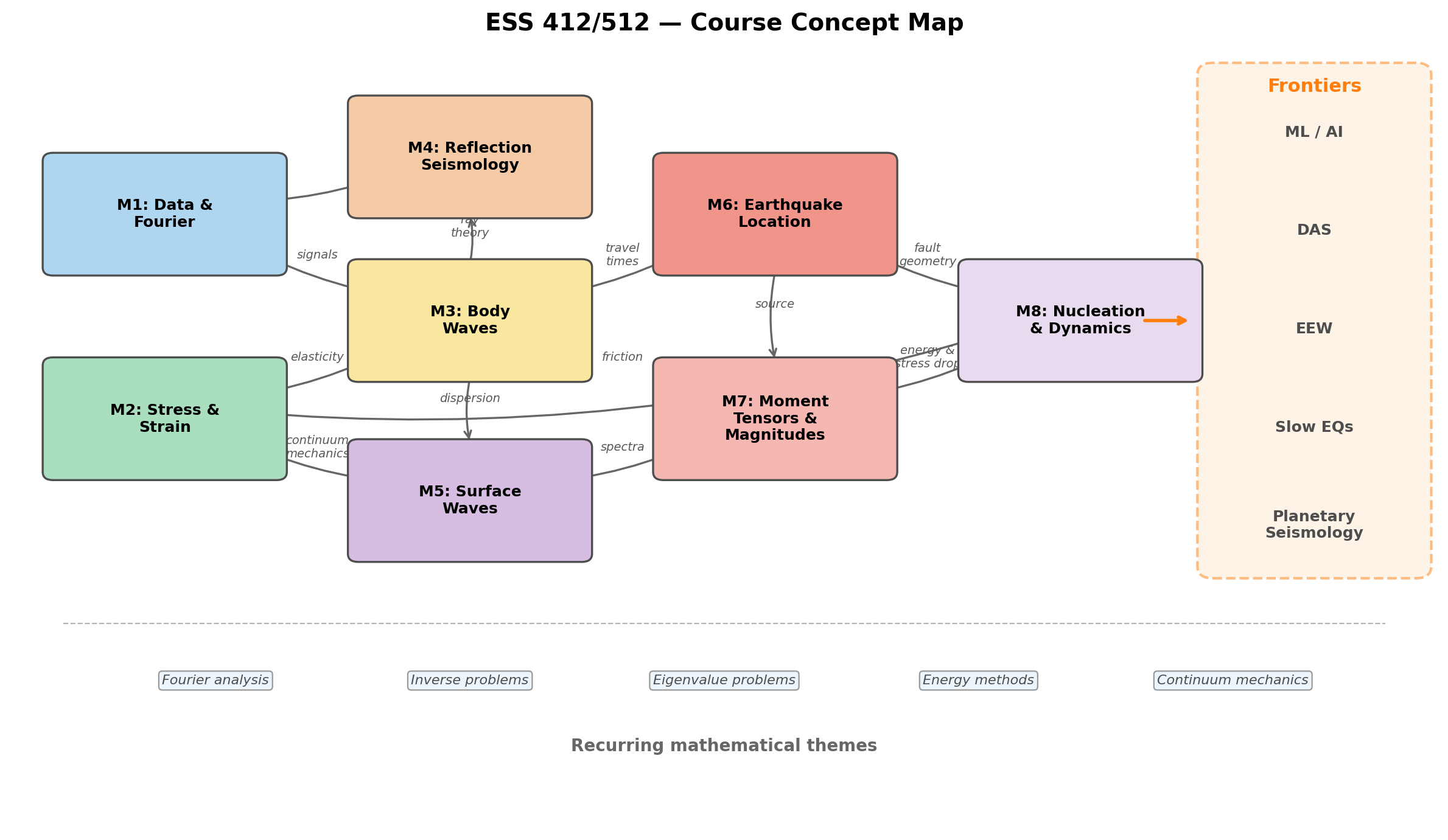
Fig. 10 Course concept map. Arrows show how each module’s concepts feed into later ones. The rightmost column previews five research frontiers discussed in §4.#
Stage |
Modules |
Core question |
|---|---|---|
Observe |
M1 (Data & Fourier) |
What does the ground actually do? |
Model the medium |
M2 (Stress & Strain), M3 (Body Waves), M4 (Reflection), M5 (Surface Waves) |
How do waves travel through the Earth? |
Locate the source |
M6 (Earthquake Location) |
Where and when did the earthquake occur? |
Characterize the source |
M7 (Moment Tensors & Magnitudes) |
How big was it, and what was the mechanism? |
Understand the physics |
M8 (Nucleation & Dynamics) |
Why did it happen, and how did it rupture? |
The narrative arc is observation → wave physics → inverse problems → source physics → fault mechanics. Each stage requires the tools developed in the previous one.
2. Recurring mathematical themes#
Five mathematical frameworks appeared repeatedly — often in disguise:
2.1 Fourier analysis#
M1: Decomposing seismograms into frequency content; instrument response as a transfer function
M4: NMO correction and migration use frequency-domain operations
M7: The source spectrum \(\hat{M}_0(\omega)\) and corner frequency \(f_c\) directly give stress drop
The convolution model above — source \(\times\) path \(\times\) instrument \(\times\) site — is the Fourier-domain backbone of the entire course.
2.2 Eigenvalue problems#
M2: Principal stresses are eigenvalues of the stress tensor \(\sigma_{ij}\)
M3: Phase velocities in anisotropic media come from the Christoffel equation (an eigenvalue problem)
M5: Surface-wave dispersion curves arise from boundary-condition eigenvalue problems
M7: Moment tensor decomposition extracts eigenvalues (isotropic, CLVD, double-couple) from \(M_{ij}\)
2.3 Inverse problems#
M4: CMP stacking and migration invert for reflector geometry
M5: Surface-wave dispersion inversion for velocity structure
M6: Earthquake location — the prototypical nonlinear geophysical inverse problem (Geiger’s method)
M7: Moment tensor inversion from first-motion polarities or waveform fitting
2.4 Energy methods#
M7: Seismic energy \(E_s\), radiated efficiency, Gutenberg–Richter energy–magnitude relation
M8: Fracture energy \(G\), energy release rate \(\mathcal{G}\), and the propagation criterion \(\mathcal{G} \geq G_c\)
2.5 Continuum mechanics#
M2: Stress, strain, Hooke’s law, Lamé parameters
M3–M5: Wave equations derived from equations of motion + constitutive law
M8: Friction laws (Coulomb, slip-weakening, rate-and-state) as constitutive relations on faults
Note
Recognizing these recurring themes is a hallmark of scientific maturity. The same eigenvalue problem that gives you principal stresses also gives you moment tensor decomposition. The same inverse-problem machinery that locates earthquakes also images Earth structure.
3. What we approximated — and what it costs us#
Every model we used made simplifying assumptions. Being explicit about them is essential for knowing when a result can be trusted.
Assumption |
Where used |
What it neglects |
|---|---|---|
Plane waves |
M3 ray theory, M4 reflection coefficients |
Near-field terms, diffraction, finite-frequency effects |
1-D Earth |
M3 global travel times, M5 dispersion |
Lateral heterogeneity, anisotropy |
Point source |
M6 location, M7 moment tensor |
Finite-fault extent, directivity |
Elastic medium |
M2–M5 wave propagation |
Attenuation (\(Q\)), anelasticity, scattering |
Homogeneous half-space |
M5 Rayleigh/Love derivation |
Layering, gradients, anisotropy |
Slip-weakening friction |
M8 nucleation |
Rate-and-state friction, thermal/fluid effects |
Warning
None of these approximations is “wrong” — they define the domain of validity. Research seismology often starts by relaxing one of these assumptions and seeing what new physics emerges.
4. Frontiers in seismology#
The five topics below are areas of intense current research. Each one directly extends concepts from our course.
4.1 Machine learning and AI in seismology#
Connection to course: M1 (signal processing), M6 (earthquake detection & location)
Traditional seismology relies on hand-crafted algorithms (STA/LTA triggers, Geiger’s method) that we implemented in labs. Deep learning replaces these with neural networks trained on millions of labeled picks.
Key developments:
PhaseNet (Zhu and Beroza [2019]): a U-Net that picks P and S arrivals from continuous waveforms, achieving human-level accuracy at machine speed
EQTransformer (Mousavi et al. [2020]): an attention-based model that simultaneously detects events and picks phases, enabling catalog construction from raw data
These tools have increased the number of detected earthquakes by 10–100× in many regions, revealing previously hidden seismicity patterns (earthquake swarms, foreshock sequences, induced seismicity).
Note
ESS 512 perspective: The mathematical backbone of these networks — convolutions, activation functions, loss minimization — is conceptually similar to the matched-filter and least-squares methods you already know. What changes is the scale of the optimization and the flexibility of the model.
4.2 Distributed Acoustic Sensing (DAS)#
Connection to course: M1 (waveform data), M3 (body waves), M5 (surface waves)
DAS converts ordinary fiber-optic telecommunication cables into dense seismic arrays with sensor spacing of ~1 m over distances of tens of kilometers (Lindsey and Martin [2021]).
How it works:
A laser interrogator sends pulses down a fiber and measures backscattered light (Rayleigh scattering)
Strain changes along the fiber shift the backscattered phase → the fiber becomes a continuous strainmeter
Typical sampling: 1-m gauge length, 1000 Hz, along 10–50 km of cable
Implications for what we learned:
M3 (body waves): DAS arrays can record teleseismic P waves at unprecedented spatial density
M5 (surface waves): Ambient-noise cross-correlation on DAS recovers surface-wave dispersion with meter-scale resolution
M4 (reflection): Urban DAS arrays are being used for shallow subsurface imaging
4.3 Earthquake Early Warning (EEW)#
Connection to course: M3 (P-wave speed > S-wave speed), M6 (real-time location), M7 (rapid magnitude estimation)
The physical basis of EEW is something you already know:
EEW systems detect the P wave in real time, estimate location and magnitude within seconds, and broadcast alerts before the damaging S and surface waves arrive (Allen and Melgar [2019]).
Key systems worldwide:
ShakeAlert (US West Coast) — operational since 2019
JMA (Japan) — operational since 2007, saved lives in the 2011 Tōhoku earthquake
SASMEX (Mexico) — one of the earliest systems, operational since 1991
Scientific challenges:
Magnitude saturation: How to estimate \(M_w\) from only the first few seconds of the P wave (connects back to M7 source spectra)
Finite-fault effects: Large earthquakes rupture for tens of seconds — the “point source” assumption (M6) breaks down
False alerts: Balancing sensitivity and specificity in noisy urban environments
4.4 Slow earthquakes and tremor#
Connection to course: M8 (friction, nucleation), M7 (moment release)
In Module 8 we derived the instability criterion for the spring-slider: slip becomes dynamic when friction weakens faster than elastic unloading. But what happens when friction weakens at nearly the same rate?
The result is slow slip — fault motion that releases tectonic stress over days to months instead of seconds (Peng and Gomberg [2010]):
Phenomenon |
Duration |
Moment rate |
|---|---|---|
Regular earthquake |
seconds |
very high |
Slow-slip event (SSE) |
days–months |
very low |
Tectonic tremor |
minutes–hours |
very low |
Low-frequency earthquake (LFE) |
~0.5 s |
low |
These phenomena form a continuum between locked faults and steady creep. They have been discovered on virtually every major subduction zone (Cascadia, Nankai, Mexico, New Zealand) and appear to interact with large megathrust earthquakes.
Note
ESS 512 perspective: The rate-and-state friction framework introduced in Module 8 naturally produces slow-slip behavior when the parameter \((a-b)\) is near zero — the boundary between velocity-weakening and velocity-strengthening friction.
4.5 Planetary seismology#
Connection to course: M2 (elastic properties), M3 (body wave travel times), M5 (surface waves)
NASA’s InSight mission placed a broadband seismometer on Mars in 2018 and recorded marsquakes until late 2022 (Banerdt et al. [2020]). This was the first sustained seismic monitoring of another planet since the Apollo lunar seismometers (1969–1977).
Key results:
Crustal thickness: ~25–50 km, constrained by receiver functions (M3 concepts)
Core: Mars has a liquid iron-alloy core with radius ~1830 km, detected via core-reflected ScS phases
Attenuation: Much higher \(Q\) in the Martian mantle than Earth → less internal heating
What transfers directly from this course:
Travel-time analysis (M3) to build a 1-D velocity model
Surface-wave dispersion (M5) for shallow structure
Moment tensor inversion (M7) — attempted for the largest marsquakes
The Moon, Europa, and Titan are next. ESA’s EnVision mission may deploy a seismometer on Venus.
5. What comes next#
If this course is the end of your seismology journey, you leave with:
The ability to read a seismogram and extract quantitative information
Fluency in the wave equation, ray theory, and inverse problems
Physical intuition for earthquake mechanics
If this is the beginning, the natural next steps are:
Computational seismology: Full-waveform simulation (spectral elements, finite differences) — see Igel [2017]
Earthquake statistics: Gutenberg–Richter, Omori’s law, ETAS models
Advanced inverse theory: Bayesian inference, adjoint methods, full-waveform inversion
Tectonophysics: Connecting seismology to geodesy, geology, and geodynamics
Check-your-understanding#
Pick any two modules and explain a mathematical concept that appears in both. Why does the same math arise in different physical contexts?
Choose one approximation from the table in §3. How would relaxing that assumption change the results of a lab you completed?
For one of the five frontiers in §4, identify which specific course concept (equation, method, or physical principle) is most directly extended by that frontier topic.
If you could add a Module 10 to this course, what would it cover and which modules would it build on?
What we deliberately did not cover#
Induced seismicity — earthquakes triggered by human activity (wastewater injection, mining, reservoir impoundment)
Seismic hazard analysis — probabilistic ground-motion prediction and building codes
Full-waveform inversion — using complete waveforms (not just travel times) to image Earth structure
Ocean-bottom seismology — instrumentation and analysis for submarine settings
Rotational seismology — measuring ground rotation in addition to translation
Reading#
📖 Shearer: Full textbook — this lecture synthesizes Chapters 1–10
Frontiers references:
Zhu and Beroza [2019] — PhaseNet: deep-learning phase picking
Mousavi et al. [2020] — EQTransformer: attention-based earthquake detection
Lindsey and Martin [2021] — Fiber-optic seismology (DAS) review
Allen and Melgar [2019] — Earthquake early warning: advances and challenges
Peng and Gomberg [2010] — The continuum between earthquakes and slow slip
Banerdt et al. [2020] — InSight mission: first results from Mars
References#
Richard M. Allen and Diego Melgar. Earthquake early warning: advances, scientific challenges, and societal needs. Annual Review of Earth and Planetary Sciences, 47:361–388, 2019. doi:10.1146/annurev-earth-053018-060457.
W. Bruce Banerdt, Suzanne E. Smrekar, Don Banfield, Domenico Giardini, Matthew Golombek, Catherine L. Johnson, Philippe Lognonné, Aymeric Spiga, Tilman Spohn, Clément Perrin, Simon C. Stähler, and Daniele Antonangeli. Initial results from the InSight mission on Mars. Nature Geoscience, 13(3):183–189, 2020. doi:10.1038/s41561-020-0544-y.
Heiner Igel. Computational Seismology: A Practical Introduction. Oxford University Press, 2017. doi:10.1093/acprof:oso/9780198717409.001.0001.
Nathaniel J. Lindsey and Eileen R. Martin. Fiber-optic seismology. Annual Review of Earth and Planetary Sciences, 49:309–336, 2021. doi:10.1146/annurev-earth-072420-065213.
S. Mostafa Mousavi, William L. Ellsworth, Weiqiang Zhu, Lindsay Y. Chuber, and Gregory C. Beroza. Earthquake transformer — an attentive deep-learning model for simultaneous earthquake detection and phase picking. Nature Communications, 11(1):3952, 2020. doi:10.1038/s41467-020-17591-w.
Zhigang Peng and Joan Gomberg. An integrated perspective of the continuum between earthquakes and slow-slip phenomena. Nature Geoscience, 3(9):599–607, 2010. doi:10.1038/ngeo940.
Weiqiang Zhu and Gregory C. Beroza. PhaseNet: a deep-neural-network-based seismic arrival-time picking method. Geophysical Journal International, 216(1):261–273, 2019. doi:10.1093/gji/ggy423.