Rayleigh Waves Theory#
Colab note: This notebook is designed to run on Google Colab. The first code cell installs dependencies.
Learning Objectives:
Derive the Rayleigh wave equation in a half-space
Understand retrograde elliptical particle motion
Analyze dispersion characteristics
Visualize depth sensitivity kernels
Prerequisites: Potential theory, Boundary value problems
Reference: Shearer, Chapter 8 (Surface Waves)
Notebook Outline:
This section designs a self-contained Python notebook that students build during or immediately after the Rayleigh-wave lecture. The goal is not numerical sophistication, but conceptual translation between:
0. Setup: parameters and nondimensionalization#
Choose β (shear speed), ν (Poisson ratio) or α/β.
Work with nondimensional phase velocity x = c/β.
beta = 3.5  # km/s (can be arbitrary scale)
nu = 0.25   # Poisson ratio (try 0.20, 0.25, 0.30, 0.33)

# From isotropic elasticity: alpha/beta = sqrt((2(1-nu))/(1-2nu))
alpha_over_beta = np.sqrt(2*(1 - nu) / (1 - 2*nu))
alpha = alpha_over_beta * beta

print(f"alpha/beta = {alpha_over_beta:.4f}")
alpha/beta = 1.7321
1. Eigenvalue problem: solve the Rayleigh equation#
Implement Rayleigh function F(x; α/β) = 0.
Root-find x in (0, 1).
# We'll solve in terms of x = c/beta in (0, 1)
# Define kappa = (beta/alpha)^2
kappa = (beta/alpha)**2

def rayleigh_F(x, kappa):
    """
    Rayleigh equation in a common dimensionless form:
      F(x) = x^6 - 8 x^4 + 8(3 - 2 kappa) x^2 - 16(1 - kappa) = 0
    where x = c/beta, kappa = (beta/alpha)^2.
    """
    x2 = x*x
    return x2**3 - 8*x2**2 + 8*(3 - 2*kappa)*x2 - 16*(1 - kappa)
plt.plot(np.linspace(0.7, 0.99, 200), [rayleigh_F(x, kappa) for x in np.linspace(0.7, 0.99, 200)])
plt.xlabel("x = c/beta")
plt.ylabel("F(x)")
plt.title("Rayleigh function F(x) vs x")
plt.grid(True)
plt.show()
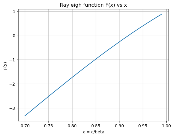
# Root bracket: Rayleigh x typically ~0.87-0.96 depending on nu.
# A safe bracket is (0.7, 0.99)
xR = brentq(rayleigh_F, 0.7, 0.99, args=(kappa,))
cR = xR * beta

print(f"Rayleigh x = cR/beta = {xR:.6f}")
print(f"Rayleigh cR = {cR:.6f} km/s")
Rayleigh x = cR/beta = 0.919402
Rayleigh cR = 3.217906 km/s
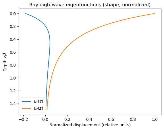
2. Eigenfunctions: depth dependence of ux(z), uz(z)#
Compute evanescence coefficients qα, qβ.
Choose amplitude ratio from boundary conditions (up to an arbitrary constant).
Plot normalized ux(z), uz(z).
For a plane wave \(exp(i(kx - wt))\) with \(c = w/k\), define:
These control exponential decay with depth: \(exp(-k q z)\)
x = xR
q_beta = np.sqrt(1 - x**2)                       # since x=c/beta
q_alpha = np.sqrt(1 - (x/alpha_over_beta)**2)    # since c/alpha = (x beta)/(alpha) = x/(alpha/beta)

# Choose wavelength to nondimensionalize depth: z' = z / lambda
# k = 2pi / lambda, so k z = 2pi (z/lambda)
lam = 1.0          # nondimensional wavelength unit
k = 2*np.pi/lam

z_over_lam = np.linspace(0, 1.5, 600)  # depth from 0 to 1.5 wavelengths
z = z_over_lam * lam
Amplitude ratio between potentials (A and B) from traction-free BCs. A full derivation yields a linear system; any non-trivial solution defines ratio.
We can enforce one boundary condition to define ratio and still get the correct shape. A commonly used ratio (up to scaling) is:
This captures the essential phase relation and nodal behavior for \(u_x\).
B_over_A = - (2*q_alpha) / (1 + q_beta**2)
Potentials (omit time and x dependence; keep depth dependence only): $\( \phi ~ A \exp(-k q_{\alpha} z), \psi ~ B exp(-k q_{\beta} z)\)$
Displacements for Rayleigh wave: $\( u_x = d\phi/dx - d\psi/dz \to (k A) \exp(-k q_{\alpha} z) + (k q_{\beta} B) \exp(-k q_{\beta} z) \)$
We’ll drop the common factor k and set A=1 for shape.
A = 1.0
B = B_over_A * A

ux = (A * np.exp(-k*q_alpha*z)) + (q_beta * B * np.exp(-k*q_beta*z))
uz = (-q_alpha * A * np.exp(-k*q_alpha*z)) + (B * np.exp(-k*q_beta*z))

# Normalize so surface vertical displacement = 1
ux /= uz[0]
uz /= uz[0]

# Plot eigenfunctions
plt.figure()
plt.plot(ux, z_over_lam, label=r"$u_x(z)$")
plt.plot(uz, z_over_lam, label=r"$u_z(z)$")
plt.gca().invert_yaxis()
plt.xlabel("Normalized displacement (relative units)")
plt.ylabel(r"Depth $z/\lambda$")
plt.title("Rayleigh-wave eigenfunctions (shape, normalized)")
plt.legend()
plt.show()
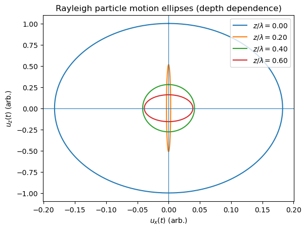
3. Particle motion#
At fixed x, build ux(t), uz(t) at selected depths.
Plot ellipses; identify retrograde vs prograde and the depth of sign change in ux.
Build time dependence: cos(ωt) and sin(ωt) phase shift. Rayleigh motion has a ~90° phase offset between ux and uz. We’ll use: $\( u_z(t) = uz(z) * cos(\omega t) \)\( \)\( u_x(t) = ux(z) * sin(\omega t) \)$
which produces an ellipse.
t = np.linspace(0, 2*np.pi, 400)

depths = [0.0, 0.2, 0.4, 0.6]  # in z/lambda
plt.figure()
for d in depths:
    idx = np.argmin(np.abs(z_over_lam - d))
    x_traj = ux[idx] * np.sin(t)
    z_traj = uz[idx] * np.cos(t)
    plt.plot(x_traj, z_traj, label=fr"$z/\lambda={z_over_lam[idx]:.2f}$")

plt.axhline(0, linewidth=0.8)
plt.axvline(0, linewidth=0.8)
# plt.gca().set_aspect("equal", adjustable="box")
plt.xlabel(r"$u_x(t)$ (arb.)")
plt.ylabel(r"$u_z(t)$ (arb.)")
plt.title("Rayleigh particle motion ellipses (depth dependence)")
plt.legend()
plt.show()
4. Sensitivity experiment#
Vary ν; re-solve cR; observe change in eigenfunctions.
sign_change_indices = np.where(np.sign(ux[:-1]) != np.sign(ux[1:]))[0]
if len(sign_change_indices) > 0:
    idx0 = sign_change_indices[0]
    print(f"ux changes sign near z/lambda ≈ {z_over_lam[idx0]:.3f} to {z_over_lam[idx0+1]:.3f}")
else:
    print("No sign change in ux found in plotted depth range.")
ux changes sign near z/lambda ≈ 0.190 to 0.193