Love Waves Theory

Love Waves Theory#

Colab note: This notebook is designed to run on Google Colab. The first code cell installs dependencies.

Learning Objectives:

Derive Love wave dispersion relation for a layer over half-space
Understand the constructive interference mechanism
Calculate phase and group velocities
Visualize mode shapes vs depth

Prerequisites: Wave equation, Eigenvalue problems

Reference: Shearer, Chapter 8 (Surface Waves)

Notebook Outline:

1. Ray picture
2. Admissible velocities and trapping condition
3. Dispersion equation (eigencondition)
4. Root finding in phase velocity
5. Dispersion curves and group velocity
6. Eigenfunctions (mode shapes)
7. Toy seismogram: dispersion → wavetrain
8. Conceptual takeaway

a low-velocity layer (β1, ρ1, thickness H) over a faster half-space (β2, ρ2).

import numpy as np
import matplotlib.pyplot as plt
from scipy.optimize import brentq

# ---- Model parameters (editable)
H_km = 20.0        # layer thickness (km)
beta1 = 3.2        # km/s (layer)
beta2 = 4.0        # km/s (half-space), must be > beta1
rho1 = 2800.0      # kg/m^3
rho2 = 3300.0      # kg/m^3

mu1 = rho1 * (beta1*1000)**2  # Pa (convert km/s to m/s)
mu2 = rho2 * (beta2*1000)**2

H = H_km * 1000.0  # m

assert beta2 > beta1, "Need beta2 > beta1 for guided Love waves in this model."

1. Ray picture#

Love waves can be viewed as constructive interference of SH surface multiples (S, SS, SSS, …).

Phase velocity: $(c = \omega/k)$ controls motion of peaks/troughs.
Group velocity: $(U = d\omega/dk)$ controls energy/envelope propagation.

Prediction questions (answer before computing):

Will Love waves be dispersive in this model? Why?
Is (U) typically less than (c) for normal Earth-like dispersion?
How will higher modes differ from the fundamental mode?

2. Admissible velocities and trapping condition#

For guided Love waves in a layer over half-space:

The phase velocity must satisfy ( \beta_1 < c < \beta_2 ).
In the layer, SH is oscillatory in depth.
In the half-space, SH must be evanescent (decay with depth).

We will enforce trapping by requiring the half-space vertical wavenumber to be real and positive decay.

def admissible_c(c):
    return (c > beta1) and (c < beta2)

3. Dispersion equation (eigencondition)#

We solve for $c$ at each angular frequency $\omega$. Let $k = \omega/c$. Define vertical wavenumbers:

Layer (oscillatory): $$ q_1 = \sqrt{\omega^2/\beta_1^2 - k^2} $$ Half-space (evanescent): $$ \kappa_2 = \sqrt{k^2 - \omega^2/\beta_2^2}$$

The Love-wave eigencondition is: $$ \tan(q_1 H) = \frac{\mu_2\,\kappa_2}{\mu_1\,q_1}. $$

Interpretation: non-trivial solutions exist only for discrete $c(\omega)$ values (modes).

def love_dispersion_F(c, omega, H, beta1, beta2, mu1, mu2):
    """
    F(c; omega) = tan(q1 H) - (mu2*kappa2)/(mu1*q1)
    Root(s) in c give Love-wave modes at frequency omega.
    """
    if not (beta1 < c < beta2):
        return np.nan

    k = omega / c

    q1_sq = (omega/beta1)**2 - k**2
    kappa2_sq = k**2 - (omega/beta2)**2

    # Trapping: q1^2 > 0 (oscillatory in layer), kappa2^2 > 0 (evanescent in half-space)
    if (q1_sq <= 0) or (kappa2_sq <= 0):
        return np.nan

    q1 = np.sqrt(q1_sq)
    kappa2 = np.sqrt(kappa2_sq)

    return np.tan(q1 * H) - (mu2 * kappa2) / (mu1 * q1)

4. Root finding in phase velocity#

At each period T (or frequency ω), solve F(c; ω)=0 in the interval (β1, β2).

Because tan() introduces multiple branches, there can be multiple roots:

fundamental mode (lowest root in ω–c sense),
higher modes (overtones).

We will:

define a frequency (period) grid,
bracket roots in c,
store multiple modes per ω (as available).

# Period grid (seconds): adjust for classroom pace
T = np.linspace(5, 80, 120)      # s
omega = 2*np.pi / T              # rad/s

# Root bracketing grid in c
c_grid = np.linspace(beta1*1.001, beta2*0.999, 2000)

def find_roots_for_omega(om, max_modes=4):
    Fvals = []
    for c in c_grid:
        Fvals.append(love_dispersion_F(c, om, H, beta1, beta2, mu1, mu2))
    Fvals = np.array(Fvals, dtype=float)

    roots = []
    # find sign changes (ignore NaNs)
    for i in range(len(c_grid)-1):
        f1, f2 = Fvals[i], Fvals[i+1]
        if np.isnan(f1) or np.isnan(f2):
            continue
        if f1 == 0:
            roots.append(c_grid[i])
        if f1*f2 < 0:
            a, b = c_grid[i], c_grid[i+1]
            try:
                r = brentq(love_dispersion_F, a, b, args=(om, H, beta1, beta2, mu1, mu2), maxiter=200)
                roots.append(r)
            except ValueError:
                pass
        if len(roots) >= max_modes:
            break
    return np.array(sorted(set(np.round(roots, 10))))

# Compute up to M modes
M = 4
c_modes = np.full((M, len(omega)), np.nan)

for j, om in enumerate(omega):
    roots = find_roots_for_omega(om, max_modes=M)
    for m in range(min(M, len(roots))):
        c_modes[m, j] = roots[m]

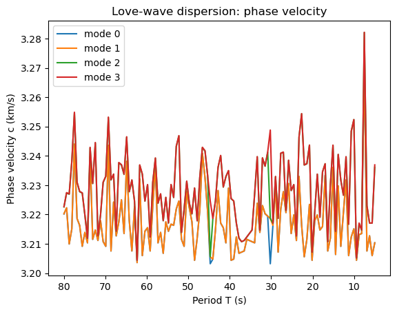
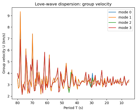
5. Dispersion curves and group velocity#

Plot phase velocity c(T) for multiple modes.

Compute group velocity from: $$ U = \frac{d\omega}{dk}, \quad k=\omega/c(\omega). $$ Numerically, compute k(ω) then differentiate.

plt.figure()
for m in range(M):
    plt.plot(T, c_modes[m], label=f"mode {m}")
plt.gca().invert_xaxis()  # optional: long period to the left
plt.xlabel("Period T (s)")
plt.ylabel("Phase velocity c (km/s)")
plt.title("Love-wave dispersion: phase velocity")
plt.legend()
plt.show()

# Group velocity estimate per mode
U_modes = np.full_like(c_modes, np.nan)
for m in range(M):
    c = c_modes[m].copy()
    valid = np.isfinite(c)
    if np.sum(valid) < 5:
        continue
    om = omega[valid]
    k = om / c[valid]  # (rad/s)/(km/s) = rad/km
    # numerical derivative: U = dω/dk
    domega = np.gradient(om)
    dk = np.gradient(k)
    U = domega / dk
    U_modes[m, valid] = U

plt.figure()
for m in range(M):
    plt.plot(T, U_modes[m], label=f"mode {m}")
plt.gca().invert_xaxis()
plt.xlabel("Period T (s)")
plt.ylabel("Group velocity U (km/s)")
plt.title("Love-wave dispersion: group velocity")
plt.legend()
plt.show()

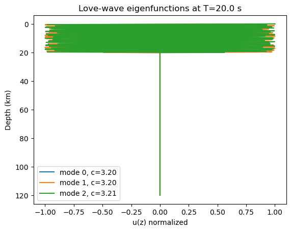
../_images/e515af8aaee0e12e0559d2b31972222e65cd2cdf8fbd31dbe186963e89160bf8.png

../_images/5030b91e047fad55fd19857ca63a5873fcb977a4b26bbe344b6c1938760b9c8a.png

6. Eigenfunctions (mode shapes)#

For a chosen period T*, and a chosen mode m:

In the layer (0 ≤ z ≤ H): u1(z) = A cos(q1 z) + B sin(q1 z)
In the half-space (z ≥ H): u2(z) = C exp(-κ2 (z-H))

Apply:

free surface traction σ_yz = 0 at z=0 → du/dz = 0 at z=0
continuity of u at z=H
continuity of traction μ du/dz at z=H

We will compute a normalized mode shape and plot u(z).

def love_mode_shape(T_star, mode_index=0, zmax_km=100.0, nz=800):
    om = 2*np.pi / T_star
    c = c_modes[mode_index, np.argmin(np.abs(T - T_star))]
    if not np.isfinite(c):
        raise ValueError("No mode available at this period for the selected mode index.")

    k = om / c
    q1 = np.sqrt((om/beta1)**2 - k**2)
    kappa2 = np.sqrt(k**2 - (om/beta2)**2)

    # From free-surface traction: du/dz(0)=0 ⇒ B=0 if we choose cos form
    # Use u1(z) = A cos(q1 z)
    A = 1.0

    # Match at z=H:
    # u1(H) = C
    # μ1 u1'(H) = μ2 u2'(H) with u2(z)=C exp(-kappa2(z-H)) ⇒ u2'(H) = -kappa2 C
    uH = A*np.cos(q1*H)
    du1H = -A*q1*np.sin(q1*H)

    # traction continuity: μ1 du1H = μ2 (-kappa2 C) = μ2 (-kappa2 uH)
    # In exact arithmetic this holds if c is a true root; we can still build shape with C=uH.
    C = uH

    z = np.linspace(0, zmax_km*1000, nz)
    u = np.zeros_like(z)

    in_layer = z <= H
    in_half = z > H

    u[in_layer] = A*np.cos(q1*z[in_layer])
    u[in_half] = C*np.exp(-kappa2*(z[in_half]-H))

    # normalize by surface amplitude
    u = u / u[0]
    return z/1000.0, u, c

# Example: choose a period and plot first few modes
T_star = 20.0
plt.figure()
for m in range(min(3, M)):
    try:
        z_km, u, c_here = love_mode_shape(T_star, mode_index=m, zmax_km=120)
        plt.plot(u, z_km, label=f"mode {m}, c={c_here:.2f}")
    except Exception:
        pass
plt.gca().invert_yaxis()
plt.xlabel("u(z) normalized")
plt.ylabel("Depth (km)")
plt.title(f"Love-wave eigenfunctions at T={T_star:.1f} s")
plt.legend()
plt.show()

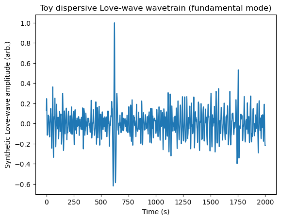
../_images/28b772287419ba30209d5fdebf834c5e2da21edf99c01fa985cd3e7278954784.png

7. Toy seismogram: dispersion → wavetrain#

We synthesize a dispersive wave packet at distance x by summing frequencies with: $$ u(x,t) = \Re \left\{ \int A(\omega)\, e^{i(k(\omega)x - \omega t)} d\omega \right\} $$ where k(ω)=ω/c(ω). The envelope arrival is controlled by group velocity U.