Surface Wave Analysis Practice#
Colab note: This notebook is designed to run on Google Colab. The first code cell installs dependencies.
Learning Objectives:
Measure group velocity dispersion from real data
Apply Frequency-Time Analysis (FTAN)
Invert dispersion curves for 1D shear velocity structure
Compare observed dispersion with theoretical models
Prerequisites: Fourier analysis, ObsPy
Reference: Shearer, Chapter 8 (Surface Waves)
Notebook Outline:
# Import libraries
import numpy as np
import matplotlib.pyplot as plt
from obspy import read, UTCDateTime
from obspy.clients.fdsn import Client
from obspy.geodetics import gps2dist_azimuth, kilometers2degrees
from obspy.signal.filter import bandpass
from scipy import signal
import warnings
warnings.filterwarnings('ignore')

# Set plotting defaults
plt.rcParams['figure.figsize'] = (12, 6)
plt.rcParams['font.size'] = 11

print("Libraries loaded successfully!")
Libraries loaded successfully!
1.2 Love Waves#
Love waves are horizontally polarized shear waves (SH motion) that propagate along the surface. They exist only in layered media (cannot exist in a homogeneous half-space).
Physical Model:#
Consider a layer of thickness \(h\) with S-wave velocity \(\beta_1\) over a half-space with velocity \(\beta_2 > \beta_1\).
Dispersion Relation (simplified):
For the fundamental mode:
where \(\beta_1 < c < \beta_2\)
The wave velocity \(c\) depends on frequency through the relationship:
where \(n\) is the mode number (0 = fundamental, 1, 2, … = higher modes).
Key Properties:#
Polarization: Horizontal motion perpendicular to propagation direction
Dispersion: Long periods (λ >> h) → \(c \rightarrow \beta_2\) (sample deeper structure)
Short periods (λ ≈ h) → \(c \rightarrow \beta_1\) (sample layer only)Fundamental vs Higher Modes: Fundamental mode has largest amplitude
Components: Strongest on transverse (T) component (E-W or N-S depending on azimuth)
# Visualize Love wave dispersion
def love_wave_dispersion(beta1, beta2, h, periods):
    """
    Simple analytical model for fundamental mode Love wave dispersion.

    Parameters:
    -----------
    beta1 : float
        S-wave velocity in layer (km/s)
    beta2 : float
        S-wave velocity in half-space (km/s)
    h : float
        Layer thickness (km)
    periods : array
        Array of periods to calculate (s)

    Returns:
    --------
    c : array
        Phase velocities (km/s)
    """
    # Simplified dispersion for demonstration
    # Real calculation requires solving transcendental equation
    wavelength = periods * beta1  # Approximate

    # Interpolate between beta1 (short period) and beta2 (long period)
    # based on wavelength/thickness ratio
    ratio = wavelength / (4 * h)
    c = beta1 + (beta2 - beta1) * (1 - np.exp(-ratio))

    # Ensure physical bounds
    c = np.clip(c, beta1, beta2)

    return c

# Example: Typical crustal structure
beta1_crust = 3.2  # km/s (crustal S velocity)
beta2_mantle = 4.5  # km/s (upper mantle S velocity)
h_crust = 35  # km (crustal thickness)

periods = np.linspace(5, 100, 96)  # 5-100 second periods
c_phase = love_wave_dispersion(beta1_crust, beta2_mantle, h_crust, periods)

# Calculate group velocity: U = dω/dk = c + k*dc/dk
# Approximate numerically
c_group = np.gradient(periods * c_phase) / np.gradient(periods)

# Plot
fig, (ax1, ax2) = plt.subplots(1, 2, figsize=(14, 5))

# Dispersion curve
ax1.plot(periods, c_phase, 'b-', linewidth=2, label='Phase Velocity')
ax1.plot(periods, c_group, 'r--', linewidth=2, label='Group Velocity')
ax1.axhline(beta1_crust, color='gray', linestyle=':', label=f'β₁ (crust) = {beta1_crust} km/s')
ax1.axhline(beta2_mantle, color='gray', linestyle=':', label=f'β₂ (mantle) = {beta2_mantle} km/s')
ax1.set_xlabel('Period (s)', fontsize=12)
ax1.set_ylabel('Velocity (km/s)', fontsize=12)
ax1.set_title('Love Wave Dispersion - Fundamental Mode', fontsize=13, fontweight='bold')
ax1.legend()
ax1.grid(True, alpha=0.3)

# Period vs wavelength
wavelength = c_phase * periods
ax2.plot(periods, wavelength, 'g-', linewidth=2)
ax2.axhline(h_crust, color='red', linestyle='--', linewidth=2, label=f'Crustal thickness = {h_crust} km')
ax2.set_xlabel('Period (s)', fontsize=12)
ax2.set_ylabel('Wavelength (km)', fontsize=12)
ax2.set_title('Wavelength vs Period', fontsize=13, fontweight='bold')
ax2.legend()
ax2.grid(True, alpha=0.3)

plt.tight_layout()
plt.show()

print(f"\nShort period (10s): c_phase = {c_phase[periods==10][0]:.2f} km/s (samples crust)")
print(f"Long period (80s): c_phase = {c_phase[periods==80][0]:.2f} km/s (samples mantle)")
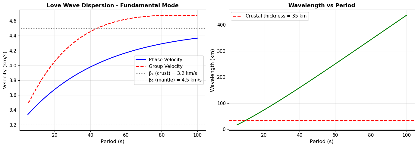
Short period (10s): c_phase = 3.47 km/s (samples crust)
Long period (80s): c_phase = 4.29 km/s (samples mantle)
1.3 Rayleigh Waves#
Rayleigh waves involve both vertical and radial motion, with particles moving in a retrograde elliptical path (opposite to wave propagation direction at the surface).
Physical Model:#
For a homogeneous half-space, Rayleigh wave velocity \(c_R\) is related to S-wave velocity \(\beta\) by:
The exact solution comes from solving the Rayleigh equation:
where \(\alpha\) is P-wave velocity and \(\beta\) is S-wave velocity.
Key Properties:#
Particle Motion: Retrograde ellipse (clockwise when looking in propagation direction)
Depth Decay: Amplitude decays exponentially with depth (e-folding ~1 wavelength)
Components: Both vertical (Z) and radial (R) components
Dispersion: In layered Earth, dispersion similar to Love waves
Velocity: Slower than both P and S waves, slightly faster than Love waves
Why Retrograde?#
The free surface boundary condition (zero stress) requires the vertical and horizontal motions to be coupled in a specific way that produces retrograde motion.
# Visualize Rayleigh wave particle motion
def rayleigh_particle_motion(depth_factor=0.2):
    """
    Simulate Rayleigh wave particle motion.

    Parameters:
    -----------
    depth_factor : float
        Depth as fraction of wavelength
    """
    # Wave parameters
    k = 2 * np.pi  # Wave number
    omega = 1.0    # Angular frequency

    # Time and position
    t = np.linspace(0, 2*np.pi, 100)
    x = 0  # Fixed position

    # Depth
    z = depth_factor * 2 * np.pi / k  # Depth as fraction of wavelength

    # Rayleigh wave displacement (simplified)
    # Vertical component
    u_z = np.exp(-k * z) * np.sin(k * x - omega * t)

    # Horizontal component (radial)
    u_r = 0.6 * np.exp(-k * z) * np.cos(k * x - omega * t)

    return u_r, u_z

# Plot particle motion at different depths
fig, axes = plt.subplots(1, 3, figsize=(15, 5))

depths = [0.0, 0.2, 0.5,1]  # Surface, 0.2λ, 0.5λ
colors = ['red', 'blue', 'green','cyan']

for ax, depth, color in zip(axes, depths, colors):
    u_r, u_z = rayleigh_particle_motion(depth)

    ax.plot(u_r, u_z, color=color, linewidth=2)
    ax.scatter([u_r[0]], [u_z[0]], color=color, s=100, zorder=5, label='Start')
    ax.arrow(u_r[10], u_z[10], u_r[11]-u_r[10], u_z[11]-u_z[10],
             head_width=0.05, head_length=0.03, fc=color, ec=color)

    ax.set_xlabel('Radial Motion (R)', fontsize=11)
    ax.set_ylabel('Vertical Motion (Z)', fontsize=11)
    ax.set_title(f'Depth = {depth:.1f}λ', fontsize=12, fontweight='bold')
    ax.axhline(0, color='gray', linestyle='--', linewidth=0.5)
    ax.axvline(0, color='gray', linestyle='--', linewidth=0.5)
    ax.set_xlim(-1, 1)
    ax.set_ylim(-1, 1)
    ax.grid(True, alpha=0.3)
    ax.set_aspect('equal')
    ax.legend()

plt.suptitle('Rayleigh Wave Particle Motion (Retrograde Ellipse)', fontsize=14, fontweight='bold', y=1.02)
plt.tight_layout()
plt.show()

print("Note: Particle motion is retrograde (clockwise) at the surface.")
print("Amplitude decreases exponentially with depth.")
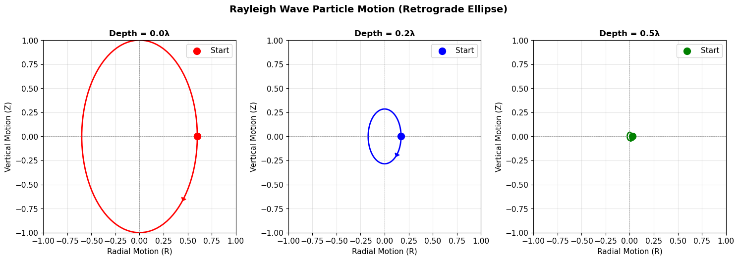
Note: Particle motion is retrograde (clockwise) at the surface.
Amplitude decreases exponentially with depth.
1.4 Dispersion: The Key to Earth Structure#
Dispersion is the phenomenon where different frequencies travel at different velocities. This is the most important property of surface waves for studying Earth structure.
Why Dispersion Occurs:#
In a layered Earth:
Long-period waves (large wavelengths) penetrate deeper → sensitive to deeper structure
Short-period waves (small wavelengths) stay shallow → sensitive to near-surface structure
Phase vs Group Velocity:#
Phase Velocity (\(c\)): Velocity of a single frequency component $\(c = \frac{\omega}{k}\)$
Group Velocity (\(U\)): Velocity of wave packet (energy propagation) $\(U = \frac{d\omega}{dk} = c + k\frac{dc}{dk}\)$
For dispersive waves: \(U \neq c\)
Physical Interpretation:
Group velocity is what we measure from arrival times
Phase velocity is what we measure from waveform correlation
For normal dispersion (typical): \(U < c\) (longer periods arrive first)
Connection to Fourier Analysis:#
This is why Notebook 02 (Fourier Transform) is a prerequisite! To measure dispersion, we must:
Decompose seismograms into frequency components (Fourier Transform)
Measure arrival time or velocity for each frequency
Plot velocity vs frequency (or period) → dispersion curve
# Demonstrate dispersion with a synthetic dispersed wave packet
def create_dispersed_waveform(distance, periods, velocities, duration=400):
    """
    Create synthetic dispersed surface wave.

    Parameters:
    -----------
    distance : float
        Distance in km
    periods : array
        Periods of components (s)
    velocities : array
        Group velocities for each period (km/s)
    duration : float
        Signal duration (s)
    """
    dt = 1.0  # 1 Hz sampling
    t = np.arange(0, duration, dt)
    signal = np.zeros_like(t)

    # Add each frequency component with its arrival time
    for T, U in zip(periods, velocities):
        omega = 2 * np.pi / T
        arrival_time = distance / U

        # Gaussian envelope
        envelope = np.exp(-((t - arrival_time) / (2*T))**2)

        # Sinusoid
        wave = envelope * np.sin(omega * (t - arrival_time))
        signal += wave

    return t, signal

# Create dispersed surface wave
distance_km = 2000  # 2000 km distance
T_range = np.array([10, 20, 40, 60])  # Different periods
U_range = love_wave_dispersion(beta1_crust, beta2_mantle, h_crust, T_range)

t, dispersed_wave = create_dispersed_waveform(distance_km, T_range, U_range)

# Plot
fig, (ax1, ax2) = plt.subplots(2, 1, figsize=(14, 8))

# Time domain
ax1.plot(t, dispersed_wave, 'k-', linewidth=0.8)
for T, U in zip(T_range, U_range):
    arrival = distance_km / U
    ax1.axvline(arrival, color='red', linestyle='--', alpha=0.5, linewidth=1.5)
    ax1.text(arrival, ax1.get_ylim()[1]*0.9, f'{T}s', ha='center', fontsize=10)

ax1.set_xlabel('Time (s)', fontsize=12)
ax1.set_ylabel('Amplitude', fontsize=12)
ax1.set_title(f'Dispersed Surface Wave Train (Distance = {distance_km} km)', fontsize=13, fontweight='bold')
ax1.grid(True, alpha=0.3)
ax1.set_xlim([400, 700])

# Spectrogram (time-frequency)
f, t_spec, Sxx = signal.spectrogram(dispersed_wave, fs=1.0, nperseg=128, noverlap=120)
im = ax2.pcolormesh(t_spec, 1/f[f>0], 10*np.log10(Sxx[f>0, :]),
                     shading='gouraud', cmap='viridis', vmin=-50, vmax=10)

# Overlay theoretical dispersion
T_theory = np.linspace(5, 100, 50)
U_theory = love_wave_dispersion(beta1_crust, beta2_mantle, h_crust, T_theory)
t_arrival_theory = distance_km / U_theory
ax2.plot(t_arrival_theory, T_theory, 'r--', linewidth=2, label='Theoretical Group Velocity')

ax2.set_xlabel('Time (s)', fontsize=12)
ax2.set_ylabel('Period (s)', fontsize=12)
ax2.set_title('Time-Frequency Representation (Spectrogram)', fontsize=13, fontweight='bold')
ax2.set_ylim([5, 80])
ax2.set_xlim([400, 700])
ax2.legend()
plt.colorbar(im, ax=ax2, label='Power (dB)')

plt.tight_layout()
plt.show()

print("\nKey Observation: Long-period waves (60s) arrive FIRST because they travel faster.")
print("This is 'normal dispersion' - typical for surface waves in continental crust.")
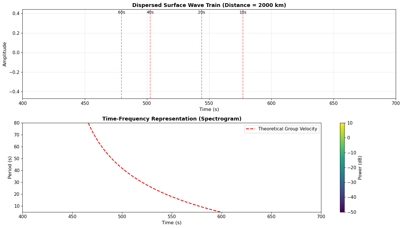
Key Observation: Long-period waves (60s) arrive FIRST because they travel faster.
This is 'normal dispersion' - typical for surface waves in continental crust.
2. ObsPy Demonstrations with Real Data#
Now we’ll work with real seismic data to identify and analyze surface waves.
2.1 Download Surface Wave Data#
For surface wave analysis, we need:
Regional to teleseismic distances (500-5000 km ideal)
Large earthquake (M > 6.0) for good signal-to-noise
Broadband seismometer data
All three components (Z, N, E) to see Love vs Rayleigh
# Initialize IRIS client
client = Client("IRIS")

# Example earthquake: 2023 Turkey-Syria M7.8
# Choose a well-recorded large earthquake
event_time = UTCDateTime("2023-02-06T01:17:35")
event_lat = 37.226
event_lon = 37.014
event_mag = 7.8
event_depth = 10.0  # km

print(f"Earthquake: M{event_mag}")
print(f"Location: {event_lat:.2f}°N, {event_lon:.2f}°E")
print(f"Time: {event_time}")
print(f"Depth: {event_depth} km")

# Download data from station in Europe (good distance for surface waves)
network = "II"  # Global Seismographic Network
station = "BFO"  # Black Forest Observatory, Germany
location = "00"
channel = "BH*"  # All broadband channels

# Time window: 30 minutes before to 2 hours after (to capture surface waves)
starttime = event_time - 30 * 60
endtime = event_time + 120 * 60

print(f"\nDownloading data from {network}.{station}...")
st = client.get_waveforms(network, station, location, channel, starttime, endtime)
print(f"Downloaded {len(st)} traces")

# Get station coordinates
inv = client.get_stations(network=network, station=station, location=location,
                          channel=channel, starttime=starttime, endtime=endtime, level="station")
station_lat = inv[0][0].latitude
station_lon = inv[0][0].longitude

# Calculate distance and azimuth
dist_m, az, baz = gps2dist_azimuth(event_lat, event_lon, station_lat, station_lon)
dist_km = dist_m / 1000.0
dist_deg = kilometers2degrees(dist_km)

print(f"\nStation: {station_lat:.2f}°N, {station_lon:.2f}°E")
print(f"Distance: {dist_km:.1f} km ({dist_deg:.2f}°)")
print(f"Azimuth: {az:.1f}°")
print(f"Back-azimuth: {baz:.1f}°")

# Basic preprocessing
st.detrend('linear')
st.taper(max_percentage=0.05)

print("\nData loaded and preprocessed successfully!")
print(st)
Earthquake: M7.8
Location: 37.23°N, 37.01°E
Time: 2023-02-06T01:17:35.000000Z
Depth: 10.0 km

Downloading data from II.BFO...
Downloaded 3 traces

Station: 48.33°N, 8.33°E
Distance: 2629.9 km (23.65°)
Azimuth: 307.1°
Back-azimuth: 107.3°

Data loaded and preprocessed successfully!
3 Trace(s) in Stream:
II.BFO.00.BHE | 2023-02-06T00:47:35.019538Z - 2023-02-06T03:17:34.969538Z | 20.0 Hz, 180000 samples
II.BFO.00.BHN | 2023-02-06T00:47:35.019538Z - 2023-02-06T03:17:34.969538Z | 20.0 Hz, 180000 samples
II.BFO.00.BHZ | 2023-02-06T00:47:35.019538Z - 2023-02-06T03:17:34.969538Z | 20.0 Hz, 180000 samples
2.2 Time-Domain Identification of Surface Waves#
Surface waves appear as large-amplitude, long-duration arrivals after the body waves.
# Plot raw seismograms
fig = plt.figure(figsize=(14, 10))

for i, tr in enumerate(st):
    ax = plt.subplot(3, 1, i+1)

    times = tr.times(type='relative', reftime=event_time)
    ax.plot(times, tr.data, 'k-', linewidth=0.5)

    # Mark expected arrivals
    p_arrival = dist_km / 8.0  # Approximate P-wave at 8 km/s
    s_arrival = dist_km / 4.5  # Approximate S-wave at 4.5 km/s
    rayleigh_arrival = dist_km / 3.5  # Approximate Rayleigh at 3.5 km/s

    ax.axvline(p_arrival, color='blue', linestyle='--', label='P (~8 km/s)', alpha=0.7)
    ax.axvline(s_arrival, color='red', linestyle='--', label='S (~4.5 km/s)', alpha=0.7)
    ax.axvline(rayleigh_arrival, color='green', linestyle='--', linewidth=2, label='Surface (~3.5 km/s)', alpha=0.7)

    ax.set_ylabel(f"{tr.stats.channel}\nAmplitude", fontsize=11)
    ax.set_xlim([0, endtime - event_time])
    ax.grid(True, alpha=0.3)
    ax.legend(loc='upper right')

    if i == 0:
        ax.set_title(f'Raw Seismograms - {network}.{station} - M{event_mag} at {dist_km:.0f} km',
                    fontsize=13, fontweight='bold')
    if i == 2:
        ax.set_xlabel('Time after origin (s)', fontsize=12)

plt.tight_layout()
plt.show()

print(f"Expected P-wave arrival: {p_arrival:.0f} s")
print(f"Expected S-wave arrival: {s_arrival:.0f} s")
print(f"Expected surface wave arrival: {rayleigh_arrival:.0f} s")
print("\nNotice: Surface waves have large amplitudes and long durations!")
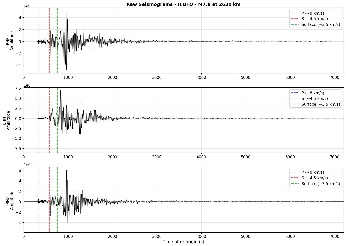
Expected P-wave arrival: 329 s
Expected S-wave arrival: 584 s
Expected surface wave arrival: 751 s

Notice: Surface waves have large amplitudes and long durations!
# Filter to isolate surface waves (0.02 - 0.1 Hz = 10-50 s period)
st_surf = st.copy()
st_surf.filter('bandpass', freqmin=0.02, freqmax=0.1, corners=4, zerophase=True)

# Plot filtered data
fig = plt.figure(figsize=(14, 10))

for i, tr in enumerate(st_surf):
    ax = plt.subplot(3, 1, i+1)

    times = tr.times(type='relative', reftime=event_time)
    ax.plot(times, tr.data, 'k-', linewidth=0.8)

    # Highlight surface wave window
    surf_start = dist_km / 3.5  # Start of surface wave window
    surf_end = dist_km / 1.5    # End of surface wave window
    ax.axvspan(surf_start, surf_end, alpha=0.2, color='green', label='Surface Wave Window')

    ax.set_ylabel(f"{tr.stats.channel}\nAmplitude", fontsize=11)
    ax.set_xlim([500, 2500])  # Zoom to surface wave arrival
    ax.grid(True, alpha=0.3)
    ax.legend(loc='upper right')

    if i == 0:
        ax.set_title(f'Bandpass Filtered (10-50s period) - Surface Waves Isolated',
                    fontsize=13, fontweight='bold')
    if i == 2:
        ax.set_xlabel('Time after origin (s)', fontsize=12)

plt.tight_layout()
plt.show()

print("Surface waves are now clearly visible!")
print("Note: Love waves (horizontal motion) vs Rayleigh waves (vertical + radial)")
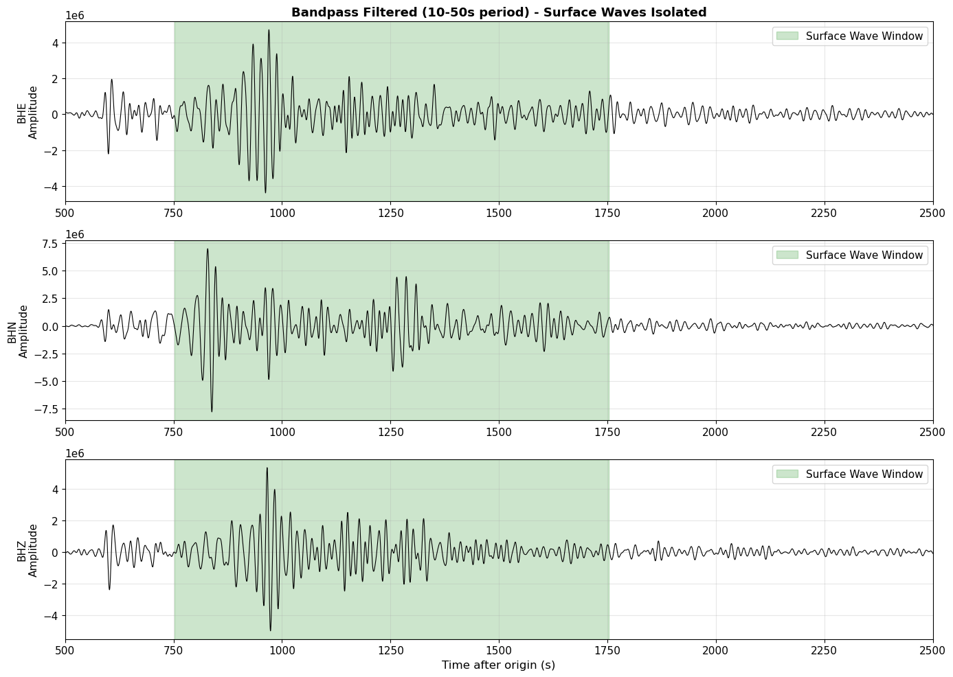
Surface waves are now clearly visible!
Note: Love waves (horizontal motion) vs Rayleigh waves (vertical + radial)
2.3 Measuring Group Velocity#
Group velocity is measured by filtering the data at different periods and measuring arrival times.
# Multiple Filter Analysis
def measure_group_velocity_mft(tr, event_time, distance_km, periods):
    """
    Measure group velocity using Multiple Filter Technique.

    Parameters:
    -----------
    tr : Trace
        Seismic trace
    event_time : UTCDateTime
        Origin time
    distance_km : float
        Distance in km
    periods : array
        Center periods for filters (s)

    Returns:
    --------
    velocities : array
        Group velocities (km/s)
    """
    velocities = []

    for T in periods:
        # Narrow bandpass around period T
        tr_filt = tr.copy()
        f_center = 1.0 / T
        f_width = 0.1 * f_center  # 10% bandwidth

        tr_filt.filter('bandpass', freqmin=f_center-f_width, freqmax=f_center+f_width,
                      corners=4, zerophase=True)

        # Find peak amplitude time (simplified - could use envelope)
        times = tr_filt.times(type='relative', reftime=event_time)

        # Search in expected surface wave window
        search_start = distance_km / 4.5  # After S-wave
        search_end = distance_km / 2.5
        mask = (times >= search_start) & (times <= search_end)

        if np.any(mask):
            idx_max = np.argmax(np.abs(tr_filt.data[mask]))
            arrival_time = times[mask][idx_max]
            U = distance_km / arrival_time
            velocities.append(U)
        else:
            velocities.append(np.nan)

    return np.array(velocities)

# Measure on vertical component (Rayleigh waves)
tr_z = st.select(channel="*Z")[0]

# Periods to analyze
periods_measure = np.array([15, 20, 25, 30, 40, 50, 60])
group_velocities = measure_group_velocity_mft(tr_z, event_time, dist_km, periods_measure)

# Plot dispersion curve
fig, ax = plt.subplots(figsize=(10, 6))

ax.plot(periods_measure, group_velocities, 'bo-', markersize=10, linewidth=2, label='Measured')

# Theoretical comparison
T_theory = np.linspace(10, 80, 50)
U_theory = love_wave_dispersion(beta1_crust, beta2_mantle, h_crust, T_theory)
ax.plot(T_theory, U_theory, 'r--', linewidth=2, label='Theoretical (simple model)')

ax.set_xlabel('Period (s)', fontsize=13)
ax.set_ylabel('Group Velocity (km/s)', fontsize=13)
ax.set_title('Surface Wave Dispersion Curve - Group Velocity', fontsize=14, fontweight='bold')
ax.legend(fontsize=11)
ax.grid(True, alpha=0.3)
ax.set_ylim([2.5, 4.5])

plt.tight_layout()
plt.show()

print("\nMeasured Group Velocities:")
for T, U in zip(periods_measure, group_velocities):
    print(f"  Period {T}s: U = {U:.2f} km/s")
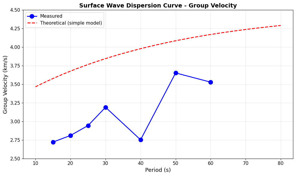
Measured Group Velocities:
  Period 15s: U = 2.72 km/s
  Period 20s: U = 2.81 km/s
  Period 25s: U = 2.94 km/s
  Period 30s: U = 3.19 km/s
  Period 40s: U = 2.75 km/s
  Period 50s: U = 3.65 km/s
  Period 60s: U = 3.53 km/s
3. Exercises#
Exercise 3.1 (ESS 412 - Undergraduate)#
Download and analyze surface waves from a different earthquake.
Choose a recent large earthquake (M > 6.5) from the past year
Download data from 3 different stations at distances between 1000-3000 km
For each station:
Calculate the distance and expected arrival times for P, S, and surface waves (assume group velocity = 3.5 km/s)
Plot the vertical component seismogram
Filter to isolate surface waves (10-50 s period)
Measure the approximate arrival time of the surface wave peak
Calculate the average group velocity
Create a table with your results:
Station name, distance, measured arrival time, calculated group velocity
Questions:
How does the measured group velocity compare to the assumed 3.5 km/s?
Do the surface waves have larger amplitude than the body waves? Why or why not?
Which component (Z, N, or E) shows the largest surface wave amplitude at each station? Can you explain why based on Love vs Rayleigh wave theory?
# Exercise 3.1 - Your code here

# Step 1: Define your earthquake
# my_event_time = UTCDateTime("...")
# ...

# Your analysis code...
Your answers to questions:
Exercise 3.2 (ESS 412 - Undergraduate)#
Particle motion analysis:
Using data from one station in Exercise 3.1:
Filter the data to isolate surface waves (10-50 s period)
Select a time window containing clear surface wave arrivals
Create particle motion plots:
Horizontal motion (N vs E) - shows Love wave polarization
Vertical vs Radial motion - shows Rayleigh wave retrograde ellipse
Hint: You’ll need to rotate horizontal components to radial/transverse using the back-azimuth.
Questions:
Can you identify retrograde motion in the vertical-radial plot?
Is the horizontal motion primarily in the transverse direction (Love wave)?
Which wave type (Love or Rayleigh) has larger amplitude at this station?
# Exercise 3.2 - Your code here
Your answers:
Exercise 3.3 (ESS 512 - Graduate)#
Complete Exercises 3.1 and 3.2, then:
Advanced Dispersion Measurement#
Implement a more sophisticated group velocity measurement:
Use the envelope function (Hilbert transform) instead of peak amplitude
Measure group velocities for periods from 10s to 80s (10 measurements)
Create a dispersion curve (group velocity vs period)
Error analysis:
Estimate uncertainty in arrival time measurements (±window size)
Propagate to uncertainty in group velocity
Plot error bars on your dispersion curve
Compare with theory:
Adjust the simple analytical model parameters (β₁, β₂, h) to fit your data
Which parameters have the strongest effect on which periods?
What crustal thickness best fits your observations?
Questions:
How does your measured dispersion compare to global average models (e.g., ak135)?
What does the dispersion tell you about crustal structure along the path?
Would you expect the same dispersion curve for a different earthquake-station pair? Why or why not?
What are the main sources of error/uncertainty in your measurements?
How could you improve the accuracy of dispersion measurements?
Your answers:
Exercise 3.4 (ESS 512 - Graduate ONLY)#
Computer Programs in Seismology (CPS) Integration#
Computer Programs in Seismology by Robert Herrmann is a comprehensive package for computing surface wave dispersion, among other things. We’ll use it to compute more accurate theoretical dispersion curves.
Installation:
# CPS can be challenging to install - see:
# http://www.eas.slu.edu/eqc/eqccps.html
# Alternative: Use Docker container or pre-compiled version
Task:
Define a realistic crustal velocity model for your earthquake-station path:
Example model (layer format: thickness, Vp, Vs, density):
10.0  5.5  3.2  2.6   # Upper crust
15.0  6.2  3.6  2.7   # Middle crust
15.0  6.8  3.9  2.9   # Lower crust
0.0   8.1  4.5  3.3   # Mantle (half-space)
Use CPS (or Python alternative like
disbaorpysurf96) to compute:Fundamental mode Love wave dispersion
Fundamental mode Rayleigh wave dispersion
Phase AND group velocities
Compare CPS predictions with your measurements from Exercise 3.3
Iterate on velocity model to improve fit
Alternative Python Packages:
disba: keurfonluu/disba (recommended)pysurf96: Python wrapper for surf96 from CPS
Questions:
How sensitive is the dispersion curve to different layer velocities?
Can you resolve crustal thickness from surface wave dispersion alone?
What periods are most sensitive to crustal vs mantle velocities?
How do Love and Rayleigh dispersion differ for the same model?
(Challenge) Read Herrmann (2013) or similar paper on CPS methodology. How do modal methods differ from ray theory for computing surface waves?
# Exercise 3.4 - Your code here

# Example with disba (if installed):
# pip install disba

# from disba import PhaseDispersion
#
# # Define velocity model
# thickness = [10.0, 15.0, 15.0, 0]  # km, 0 = half-space
# vp = [5.5, 6.2, 6.8, 8.1]  # km/s
# vs = [3.2, 3.6, 3.9, 4.5]  # km/s
# rho = [2.6, 2.7, 2.9, 3.3]  # g/cm³
#
# # Compute Love wave dispersion
# pd = PhaseDispersion(*np.array([thickness, vp, vs, rho]))
# periods = np.logspace(0, 2, 50)  # 1-100 s
# love_phase = pd(periods, mode=0, wave="love")
#
# # Plot...

# Your code here...
Your answers and model:
Summary and Connections#
Key Takeaways:#
Surface waves (Love, Rayleigh) propagate along Earth’s surface and are dispersive in layered media
Dispersion means different frequencies travel at different velocities → probe different depths
Group velocity (energy propagation) ≠ phase velocity (wavefront) for dispersive waves
Long periods sample deeper structure; short periods sample shallow structure
Measuring dispersion curves allows us to invert for Earth’s velocity structure
Connections to Other Topics:#
Notebook 02 (Fourier): Dispersion analysis requires frequency decomposition
Notebook 03 (Ray Theory): Body waves follow rays; surface waves are modal
Notebook 06 (Noise Correlation): Surface waves dominate ambient seismic noise → can extract Green’s functions
Real Research: Surface wave tomography maps crustal/mantle structure globally and regionally
Further Reading:#
Shearer, P. (2019). Introduction to Seismology, 3rd Ed., Chapter 7
Aki, K., & Richards, P. G. (2002). Quantitative Seismology, Chapters 7-8
Stein & Wysession (2003). An Introduction to Seismology, Earthquakes, and Earth Structure, Chapter 3
Herrmann, R. B. (2013). Computer programs in seismology: An evolving tool for instruction and research. Seismological Research Letters, 84(6), 1081-1088.
Research Applications:#
Regional Tomography: Lin et al. (2008) using ambient noise
Crustal Thickness: Moschetti et al. (2007) for western US
Earthquake Early Warning: Allen & Melgar (2019) - surface waves used for rapid magnitude
Basin Effects: Graves et al. (1998) - Los Angeles basin amplification
End of Notebook 05