![]()
Note: If running on Colab, uncomment and run the pip install cell below.
Lab 7d: STF, Spectra & Energy Budget#
Learning Objectives#
Generate synthetic source time functions (STFs) and compute their spectra.
Observe how rupture directivity biases inferred corner frequency \(f_c\) with azimuth.
Quantify how a two-pulse (complex) STF changes spectral estimates of stress drop.
Compute a proxy radiated energy \(E_R\) and apparent stress \(\sigma_a = \mu E_R / M_0\).
Explore the earthquake energy budget sandbox and connect radiation efficiency \(\eta_R\) to the “missing energy” problem.
Prerequisites#
Lecture: Earthquake Source Dynamics (07d)
Lecture: Earthquake Magnitudes (07c)
Estimated Completion Time#
~60 minutes
import numpy as np
import matplotlib.pyplot as plt

# ── figure defaults ──────────────────────────────────────────────────────────
plt.rcParams.update({
    "figure.dpi": 110,
    "axes.grid": True,
    "grid.alpha": 0.3,
    "font.size": 11,
    "axes.titlesize": 12,
})

# ── helper functions ─────────────────────────────────────────────────────────

def next_pow2(n):
    """Return the smallest power of 2 >= n."""
    return int(2 ** np.ceil(np.log2(max(n, 1))))


def rfft(x, dt):
    """One-sided real FFT.  Returns (freq, complex_spectrum)."""
    X = np.fft.rfft(x)
    f = np.fft.rfftfreq(len(x), d=dt)
    return f, X


def brune_stf(t, M0=1.0, fc=0.25, t0=0.0):
    """Brune (1970) moment-rate function, normalized so integral = M0.

    Parameters
    ----------
    t  : array  — time axis (s)
    M0 : float  — scalar moment (arb. units)
    fc : float  — corner frequency (Hz)
    t0 : float  — onset time (s)
    """
    tt = np.clip(t - t0, 0, None)
    Mdot = (2 * np.pi * fc) ** 2 * tt * np.exp(-2 * np.pi * fc * tt)
    norm = np.trapezoid(Mdot, t)
    return M0 * Mdot / (norm + 1e-30)


def two_pulse_stf(t, M0=1.0, fc=0.25, dt_sep=3.0, frac=0.35):
    """Two-pulse (complex) STF: main pulse + delayed secondary pulse.

    Parameters
    ----------
    dt_sep : float — temporal separation between pulses (s)
    frac   : float — fraction of M0 in the secondary pulse
    """
    M1 = brune_stf(t, M0=1.0, fc=fc, t0=0.0)
    M2 = brune_stf(t, M0=1.0, fc=1.8 * fc, t0=dt_sep)
    Mdot = (1 - frac) * M1 + frac * M2
    norm = np.trapezoid(Mdot, t)
    return M0 * Mdot / (norm + 1e-30)


def directivity_warp(Mdot_ref, t, Vr_over_c=0.6, theta_deg=0.0):
    """Apply toy Doppler directivity: rescale time axis by (1 - Vr/c * cos θ).

    Moment is conserved by dividing by the scale factor.
    """
    scale = max(1.0 - Vr_over_c * np.cos(np.deg2rad(theta_deg)), 0.05)
    Mdot_warped = np.interp(t / scale, t, Mdot_ref, left=0.0, right=0.0)
    return Mdot_warped / scale


def estimate_fc(f, A):
    """Crude corner-frequency estimate: where amplitude drops to plateau/√2."""
    plateau = np.median(A[1:6])
    target = plateau / np.sqrt(2)
    idx = np.where(A[1:] <= target)[0]
    return float("nan") if len(idx) == 0 else float(f[1:][idx[0]])


def stress_drop_brune(M0, fc, beta=3500.0, k=0.37):
    """Brune stress drop and source radius from M0 and fc.

    Returns (delta_sigma [Pa], r [m]) using r = k * beta / fc.
    """
    r = k * beta / (fc + 1e-30)
    dsg = (7 / 16) * M0 / (r ** 3 + 1e-30)
    return dsg, r


def ricker(t, f0=1.0):
    """Ricker wavelet centred at t=0 with peak frequency f0 Hz."""
    a = (np.pi * f0 * t) ** 2
    return (1 - 2 * a) * np.exp(-a)


def convolve_same(x, h, dt):
    """Linear convolution with 'same' length, scaled by dt."""
    return np.convolve(x, h, mode="same") * dt


def radiated_energy_proxy(v, dt):
    """Proxy radiated energy ∝ ∫ v(t)² dt."""
    return float(np.trapezoid(v ** 2, dx=dt))


print("Setup complete.")
Setup complete.
1. Omega-square model: the reference STF#
Predict (before running): Sketch what \(\dot{M}(t)\) looks like for the Brune model. How does increasing \(f_c\) change (a) the duration of the STF and (b) the corner in the spectrum?
dt = 0.01           # s  — time step
t = np.arange(-5, 35, dt)
M0 = 1.0            # arb. moment units

fc_values = [0.15, 0.25, 0.50]   # Hz
fig, (ax1, ax2) = plt.subplots(1, 2, figsize=(11, 4))

for fc in fc_values:
    Mdot = brune_stf(t, M0=M0, fc=fc, t0=0.0)
    ax1.plot(t, Mdot, label=f"$f_c$ = {fc} Hz")

    n = next_pow2(len(Mdot))
    f, X = rfft(np.pad(Mdot, (0, n - len(Mdot))), dt)
    ax2.loglog(f[1:], np.abs(X[1:]), label=f"$f_c$ = {fc} Hz")

ax1.set_xlabel("Time (s)")
ax1.set_ylabel("Moment rate (arb.)")
ax1.set_title("Brune STF — time domain")
ax1.set_xlim(-0.5, 20)
ax1.legend()

ax2.set_xlabel("Frequency (Hz)")
ax2.set_ylabel("$|\\dot{M}(f)|$ (arb.)")
ax2.set_title("Source spectrum")
ax2.legend()

plt.tight_layout()
plt.show()
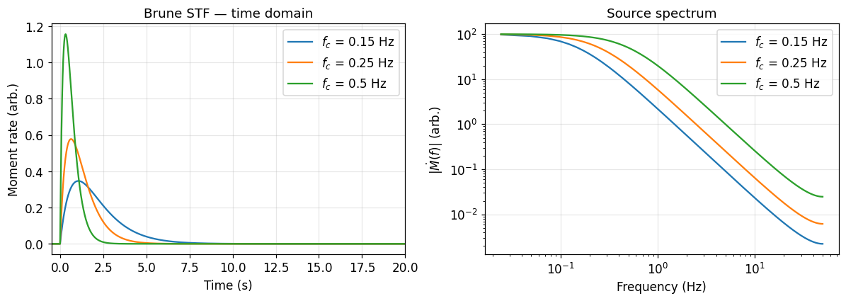
Explain & Check:
Does a higher \(f_c\) produce a shorter or longer STF? Confirm with the plot.
Mark the corner frequency on the log-log spectrum. What is the slope above \(f_c\)?
The low-frequency plateau is the same for all curves. What seismic parameter does it represent?
2. Directivity: how \(V_r\) biases \(f_c\) and apparent stress drop#
Predict (before running): For a rupture propagating at \(V_r = 0.6\,c\):
In which azimuth does the STF appear shorter?
If you estimate \(f_c\) without knowing the source direction, which station will infer the largest stress drop? Why?
fc0 = 0.25
Mdot0 = brune_stf(t, M0=M0, fc=fc0, t0=0.0)   # reference STF (no directivity)

Vr_over_c = 0.6
thetas = [0, 60, 120, 180]                      # deg from rupture direction

# Apply directivity warp and compute spectra + stress-drop estimates
Mdots, spectra = {}, {}
for th in thetas:
    md = directivity_warp(Mdot0, t, Vr_over_c=Vr_over_c, theta_deg=th)
    Mdots[th] = md
    n = next_pow2(len(md))
    f, X = rfft(np.pad(md, (0, n - len(md))), dt)
    A = np.abs(X)
    fc_hat = estimate_fc(f, A)
    dsg, r = stress_drop_brune(M0, fc_hat)
    spectra[th] = dict(f=f, A=A, fc=fc_hat, dsg=dsg, r=r)

# ── Time-domain plot ──────────────────────────────────────────────────────────
fig, (ax1, ax2) = plt.subplots(1, 2, figsize=(11, 4))
for th in thetas:
    ax1.plot(t, Mdots[th], label=f"θ = {th}°")
ax1.set_xlim(-0.5, 20)
ax1.set_xlabel("Time (s)")
ax1.set_ylabel("Moment rate (arb.)")
ax1.set_title("Directivity-warped STF")
ax1.legend()

for th in thetas:
    s = spectra[th]
    ax2.loglog(s["f"][1:], s["A"][1:], label=f"θ={th}°, $f_c$≈{s['fc']:.2f} Hz")
ax2.set_xlabel("Frequency (Hz)")
ax2.set_ylabel("$|\\dot{M}(f)|$ (arb.)")
ax2.set_title("Spectra with directivity")
ax2.legend()
plt.tight_layout()
plt.show()

# ── Summary table ─────────────────────────────────────────────────────────────
print(f"{'θ (°)':>6}  {'fc_hat (Hz)':>12}  {'Δσ_toy (arb.)':>14}  {'r_toy (m)':>10}")
for th in thetas:
    s = spectra[th]
    print(f"{th:>6}  {s['fc']:>12.3f}  {s['dsg']:>14.3e}  {s['r']:>10.1f}")
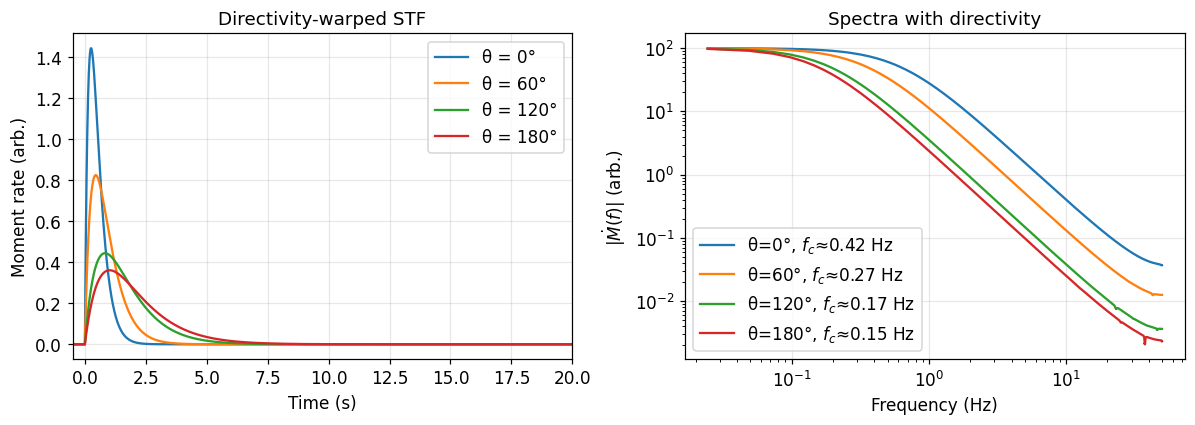
 θ (°)   fc_hat (Hz)   Δσ_toy (arb.)   r_toy (m)
     0         0.415       1.440e-11      3120.2
    60         0.269       3.902e-12      4822.1
   120         0.171       1.006e-12      7577.6
   180         0.146       6.332e-13      8840.5
Explain & Check:
By what factor does the inferred stress drop differ between \(\theta = 0°\) and \(\theta = 180°\)? Is this consistent with the cubic \(f_c^3\) dependence?
The long-period plateau (\(M_0\)) should be the same for all azimuths. Is it?
What single observation — without knowing source direction — would tell you directivity is present?
3. STF complexity: two pulses, one biased spectrum#
Predict (before running): A second sub-event adds energy at a later time. Do you expect the composite spectrum to show a higher or lower apparent \(f_c\) compared with a single-pulse STF with the same \(M_0\)? Why might this matter for cataloging stress drops?
Mdot_simple = brune_stf(t, M0=M0, fc=0.25, t0=0.0)
Mdot_complex = two_pulse_stf(t, M0=M0, fc=0.25, dt_sep=3.0, frac=0.35)

def get_spectrum(md):
    n = next_pow2(len(md))
    f, X = rfft(np.pad(md, (0, n - len(md))), dt)
    A = np.abs(X)
    return f, A, estimate_fc(f, A)

f1, A1, fc1 = get_spectrum(Mdot_simple)
f2, A2, fc2 = get_spectrum(Mdot_complex)

fig, (ax1, ax2) = plt.subplots(1, 2, figsize=(11, 4))

ax1.plot(t, Mdot_simple, label="Simple (single pulse)")
ax1.plot(t, Mdot_complex, label="Complex (two pulses)")
ax1.set_xlim(-0.5, 20)
ax1.set_xlabel("Time (s)")
ax1.set_ylabel("Moment rate (arb.)")
ax1.set_title("STF comparison")
ax1.legend()

ax2.loglog(f1[1:], A1[1:], label=f"Simple  $f_c$ ≈ {fc1:.2f} Hz")
ax2.loglog(f2[1:], A2[1:], label=f"Complex $f_c$ ≈ {fc2:.2f} Hz")
ax2.set_xlabel("Frequency (Hz)")
ax2.set_ylabel("$|\\dot{M}(f)|$ (arb.)")
ax2.set_title("Spectral impact of complexity")
ax2.legend()
plt.tight_layout()
plt.show()

print(f"Simple  fc = {fc1:.3f} Hz | Complex fc = {fc2:.3f} Hz")
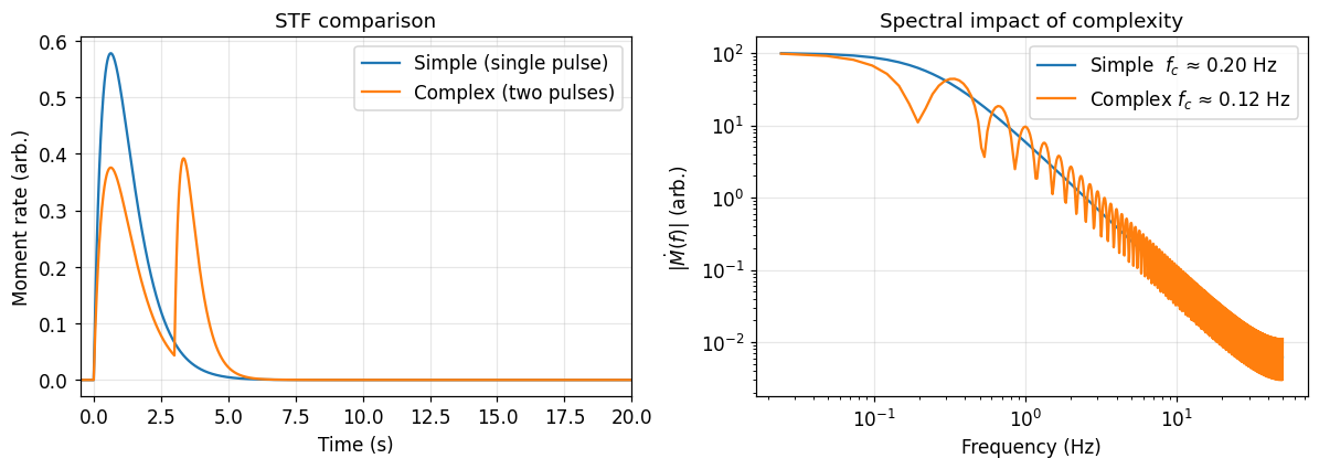
Simple fc = 0.195 Hz | Complex fc = 0.122 Hz
Explain & Check:
Does complexity cause the single-corner estimate to be biased high or low?
Describe one observational test that could distinguish a truly higher-stress-drop event from a complex rupture with a biased \(f_c\) estimate.
How does this relate to the finding of Neely et al. (2024) about magnitude trends in \(\Delta\sigma\)?
4. Radiated energy proxy and apparent stress#
We convolve each STF with a simple Ricker wavelet (proxy Green’s function) to get a toy far-field velocity seismogram, then compute:
Predict (before running): Which should show higher \(E_R\): the complex or the simple STF? Which directivity azimuth — forward or backward — should yield higher \(E_R\)?
g = ricker(t, f0=1.0)
g /= np.max(np.abs(g))
mu = 30e9  # Pa — rigidity

def toy_seismo(Mdot):
    """Convolve STF with Ricker wavelet → displacement u; differentiate → velocity v."""
    u = convolve_same(Mdot, g, dt)
    v = np.gradient(u, dt)
    return u, v

cases = {
    "Simple": Mdot_simple,
    "Complex": Mdot_complex,
    "Forward (θ=0°)": Mdots[0],
    "Backward (θ=180°)": Mdots[180],
}

results = {}
fig, ax = plt.subplots(figsize=(9, 4))
for label, Mdot in cases.items():
    u, v = toy_seismo(Mdot)
    ER = radiated_energy_proxy(v, dt)
    sa = mu * ER / M0
    results[label] = dict(ER=ER, sa=sa)
    ax.plot(t, v, label=label)

ax.set_xlim(-1, 20)
ax.set_xlabel("Time (s)")
ax.set_ylabel("Toy velocity (arb.)")
ax.set_title("Far-field velocity proxy")
ax.legend()
plt.tight_layout()
plt.show()

print(f"{'Case':<22}  {'ER (arb.)':>12}  {'σ_a (arb.)':>12}")
for label, r in results.items():
    print(f"{label:<22}  {r['ER']:>12.3e}  {r['sa']:>12.3e}")
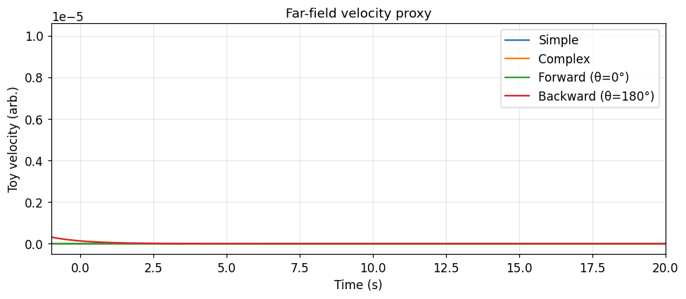
Case                       ER (arb.)    σ_a (arb.)
Simple                     4.377e-14     1.313e-03
Complex                    2.247e-14     6.741e-04
Forward (θ=0°)             1.396e-30     4.188e-20
Backward (θ=180°)          6.044e-11     1.813e+00
Explain & Check:
Does \(E_R\) depend on source complexity or just \(M_0\)? Interpret the numbers.
Why does the forward station record higher \(E_R\) despite experiencing the same seismic moment?
\(\sigma_a\) uses a proxy here (not real units). What would you need for a physical measurement?
5. Energy budget sandbox#
We use the radiation efficiency \(\eta_R\) to explore the energy balance:
Predict (before running): If \(\eta_R\) drops from 0.5 to 0.1, how does the “missing energy” (fracture + heat) change relative to \(E_R\)?
ER_ref = results["Simple"]["ER"]   # use simple STF proxy as reference
etas = [0.80, 0.50, 0.25, 0.10, 0.05]

print(f"Reference ER = {ER_ref:.3e} (arb.)")
print()
print(f"{'η_R':>6}  {'ΔE_strain':>12}  {'E_missing (G+H)':>16}  {'E_missing / ER':>14}")
for eta in etas:
    E_strain = ER_ref / eta
    E_miss = E_strain - ER_ref
    print(f"{eta:>6.2f}  {E_strain:>12.3e}  {E_miss:>16.3e}  {E_miss/ER_ref:>14.1f}×")
Reference ER = 4.377e-14 (arb.)

   η_R     ΔE_strain   E_missing (G+H)  E_missing / ER
  0.80     5.471e-14         1.094e-14             0.2×
  0.50     8.754e-14         4.377e-14             1.0×
  0.25     1.751e-13         1.313e-13             3.0×
  0.10     4.377e-13         3.939e-13             9.0×
  0.05     8.754e-13         8.316e-13            19.0×
Wrap-up: putting it all together#
Answer the following questions in the cells below or in your notebook:
Directivity bias: In this exercise, \(V_r / c = 0.6\). Compute the theoretical ratio \(f_{c,\text{forward}} / f_{c,\text{backward}}\) from the Doppler formula and compare it to the ratio you measured from the spectra.
Cubic amplification: From your directivity table, pick the worst-case azimuth. What is the ratio of apparent stress drops \(\Delta\sigma_\text{forward} / \Delta\sigma_0\)? Verify it equals \((f_{c,\text{forward}} / f_{c,0})^3\).
Complexity vs directivity: The complex STF and the forward-directed STF both show elevated \(f_c\). Describe an observational strategy to distinguish them in a real dataset.
Energy budget: If you measure \(M_w = 5.0\) (\(M_0 \approx 3.6 \times 10^{16}\) N·m), \(\Delta\sigma = 3\) MPa, and \(\eta_R = 0.06\) (a typical natural earthquake value), estimate \(E_R\), \(\Delta E_\text{strain}\), and \(E_G + E_H\). Assume \(\beta = 3500\) m/s, \(\mu = 30\) GPa, \(\rho = 2700\) kg/m³.