Ray Theory I: Snell’s Law and the Ray Parameter

Ray Theory I: Snell’s Law and the Ray Parameter#

Learning objectives#

After this lecture, students should be able to:

Explain why seismic rays bend in layered media using travel-time arguments.
Define and interpret the ray parameter ( p ) physically and geometrically.
Predict qualitative ray paths in velocity structures that increase with depth.
Relate ray geometry to observable quantities such as travel-time curves.

Context and scope#

This lecture introduces the conceptual core of ray theory. We focus on geometry and timing, not amplitudes or full wavefields.

Ray theory is a high-frequency approximation: it describes where energy travels, not how waveforms interfere. Despite its limitations, it underpins:

Earthquake location
1-D and 3-D travel-time tomography
Phase identification at local and global scales

This material corresponds primarily to Shearer (2009), Chapter 4.1–4.2.

1. Plane waves and interfaces: the physical picture#

Consider a plane seismic wave propagating through a homogeneous medium. Wavefronts are surfaces of constant phase, and rays are normal to wavefronts.

When such a wave encounters a horizontal interface, two constraints must be satisfied:

Continuity of arrival time along the interface
Stationarity of total travel time between source and receiver (Fermat’s principle)

These constraints force rays to bend.

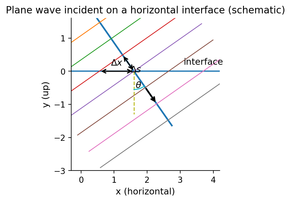
Schematic of a plane wave incident on a horizontal interface showing ray angle and wavefront spacing — Fig. 1 Plane wave incident on a horizontal interface. The ray angle θ is measured from vertical, and wavefront spacing Δs relates to horizontal spacing Δx through the ray parameter.#

2. Derivation of Snell’s law (seismological form)#

Let:

$v$ be seismic velocity
$u = 1/v$ be slowness
$\theta$ be the ray angle measured from vertical

From geometry of successive wavefronts:

\[p \equiv \frac{\sin\theta}{v} = u \sin\theta\]

This quantity $p$ is called the ray parameter.

Across a horizontal interface:

\[ u_1 \sin\theta_1 = u_2 \sin\theta_2 = p\]

This is Snell’s law, written in seismological form.

📖 Shearer reference: Fig. 4.2 (Snell’s law across layers)

Physical interpretation (critical)#

The ray parameter $p$:

Is the horizontal slowness of the wave
Equals the slope of the travel-time curve: $$ p = \frac{dT}{dX}$$
Is conserved only in laterally homogeneous media

This is why ray theory works so naturally for layered Earth models.

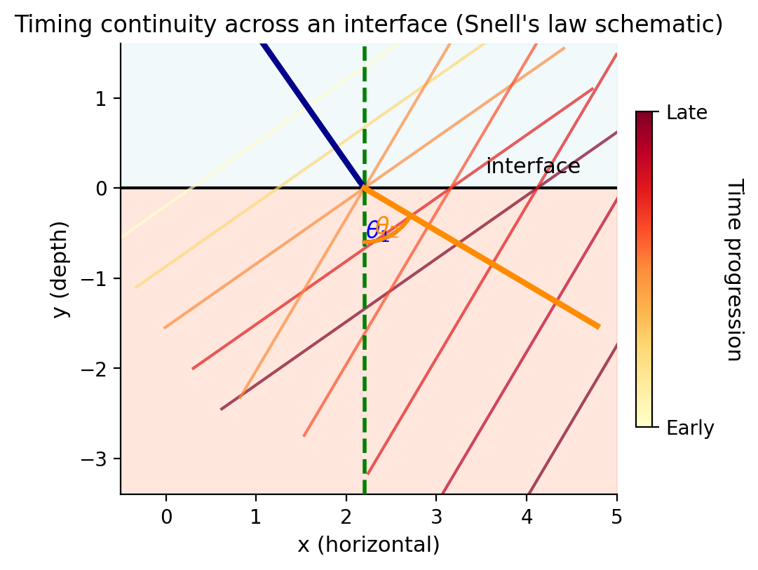
Wavefronts crossing an interface between two layers with different velocities — Fig. 2 Snell’s law as timing continuity. Wavefronts (colored by time progression from early to late) bend across the interface, preserving arrival time continuity. The ray parameter p = u sin θ remains constant across the boundary.#

3. Rays in media with velocity increasing with depth#

In the Earth, both $ V_P $ and $ V_S $ generally increase with depth.

Because $ p = u \sin\theta $ is constant:

As $ u $ decreases with depth
$ \sin\theta $ must increase
Rays bend away from vertical

Eventually, $ \theta = 90^\circ $, defining a turning point.

📖 Shearer reference: Fig. 4.3 (curved rays and turning points)

Key consequences#

Steep rays (small $ p $) turn deeper
Shallow rays (large $ p $) turn near the surface
Far-offset arrivals sample deeper Earth structure

This single idea explains why travel-time curves encode depth information.

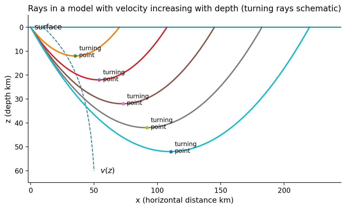
Curved ray paths in a velocity model increasing with depth — Fig. 3 Ray paths in a model with velocity increasing with depth. Rays with different takeoff angles (different ray parameters p) turn at different depths. Steeper rays (smaller p) penetrate deeper before returning to the surface.#

4. Ray parameter and travel-time curves#

Each observed arrival at distance $ X $ corresponds to one ray with a specific $ p $.

Plotting first-arrival time versus distance produces a travel-time curve:

\[ T(X)\]

The slope at any point is:

\[ \frac{dT}{dX} = p\]

📖 Shearer reference: Fig. 4.4 (travel-time curve and ray parameter)

Conceptual inversion#

Observations: $ T(X) $
Slopes give: $ p(X) $
Geometry + physics link $ p $ to turning depth

This is the foundation of travel-time inversion.

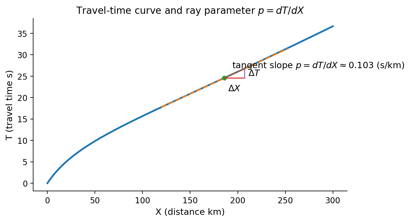
Travel-time curve with tangent line showing ray parameter — Fig. 4 Travel-time curve T(X) and ray parameter. The slope of the tangent line at any point equals the ray parameter: p = dT/dX. This geometric relationship connects observable travel times to ray paths.#

5. Check-your-understanding (conceptual)#

Q1. Two P-wave arrivals are recorded at different distances. One has a smaller $ dT/dX $ than the other.
- Which ray turned deeper?
- Which ray sampled higher velocities?
Q2. If velocity were constant with depth, would rays ever return to the surface? Why or why not?
Q3. Why is $ p $ no longer constant in laterally varying velocity models?

Students should answer these before seeing numerical ray tracing.

What we deliberately did not do#

No full derivation from the eikonal equation
No amplitudes, caustics, or head waves yet
No spherical geometry yet

Looking ahead#

Next, we will:

Turn these ideas into numerical ray tracing
Explore when ray theory fails (LVZs, triplications)
Extend the ray parameter concept to the spherical Earth

Reading#

Shearer, P. M. (2009), Introduction to Seismology, 2nd ed. Chapter 4.1–4.2 (Snell’s law and ray paths)