Stress, Strain, and the Equation of Motion

Stress, Strain, and the Equation of Motion#

1. The Geoscientific Question#

When a magnitude 8 earthquake ruptures the Cascadia subduction zone, the ground in Seattle will shake within two minutes. That shaking arrives as waves — not water waves, not sound waves, but elastic waves: mechanical disturbances that travel through rock by momentarily deforming it. No mass moves from Cascadia to Seattle; only a pattern of stress and strain propagates.

The speed at which this energy arrives — and how violent the shaking will be — depends on the elastic properties of every rock unit the waves travel through: the oceanic crust of the Juan de Fuca plate, the mantle wedge above it, the accreted terranes of the Coast Range, and the soft Seattle Basin sediments beneath the city. To use seismograms to image any of those structures, we first need a precise mathematical description of what elastic deformation is and how it propagates.

This lecture builds that description from the ground up. The governing physics is continuum mechanics: the mechanics of deformable solids treated as continuous fields of stress and strain. The mathematical tools are tensors and partial differential equations. The payoff is the equation of motion — a wave equation whose coefficients are the very material properties we want to measure.

The Central Question

How does the elastic response of rock to applied stress give rise to waves whose speed we can measure from a seismogram?

2. Governing Physics: Elastic Deformation#

2.1 The Linear Elastic Assumption#

When a seismic wave passes through rock, it deforms the rock and then the rock springs back. This is elastic behavior: deformation is fully recoverable once the stress is removed. The additional assumption that makes the mathematics tractable is linearity: stress is proportional to strain.

This linear elastic (Hookean) regime applies when strains are small — roughly below $10^{-4}$. Typical seismic strains are $10^{-6}$ to $10^{-8}$, well inside the linear regime. The assumption breaks down near fault zones (permanent deformation), in partially molten rock (viscous flow), and at the very high pressures of the deep mantle (nonlinear response). For the purposes of seismic wave propagation through intact rock, it is an excellent approximation.

Key Concept: Elastic Deformation

Seismic wave propagation relies on two linked assumptions: (1) the rock is elastic — it returns to its original shape after deformation — and (2) the relationship between stress and strain is linear. These are collectively called Hookean elasticity. Seismic strains ($\sim 10^{-7}$) are tiny enough that this is almost always valid.

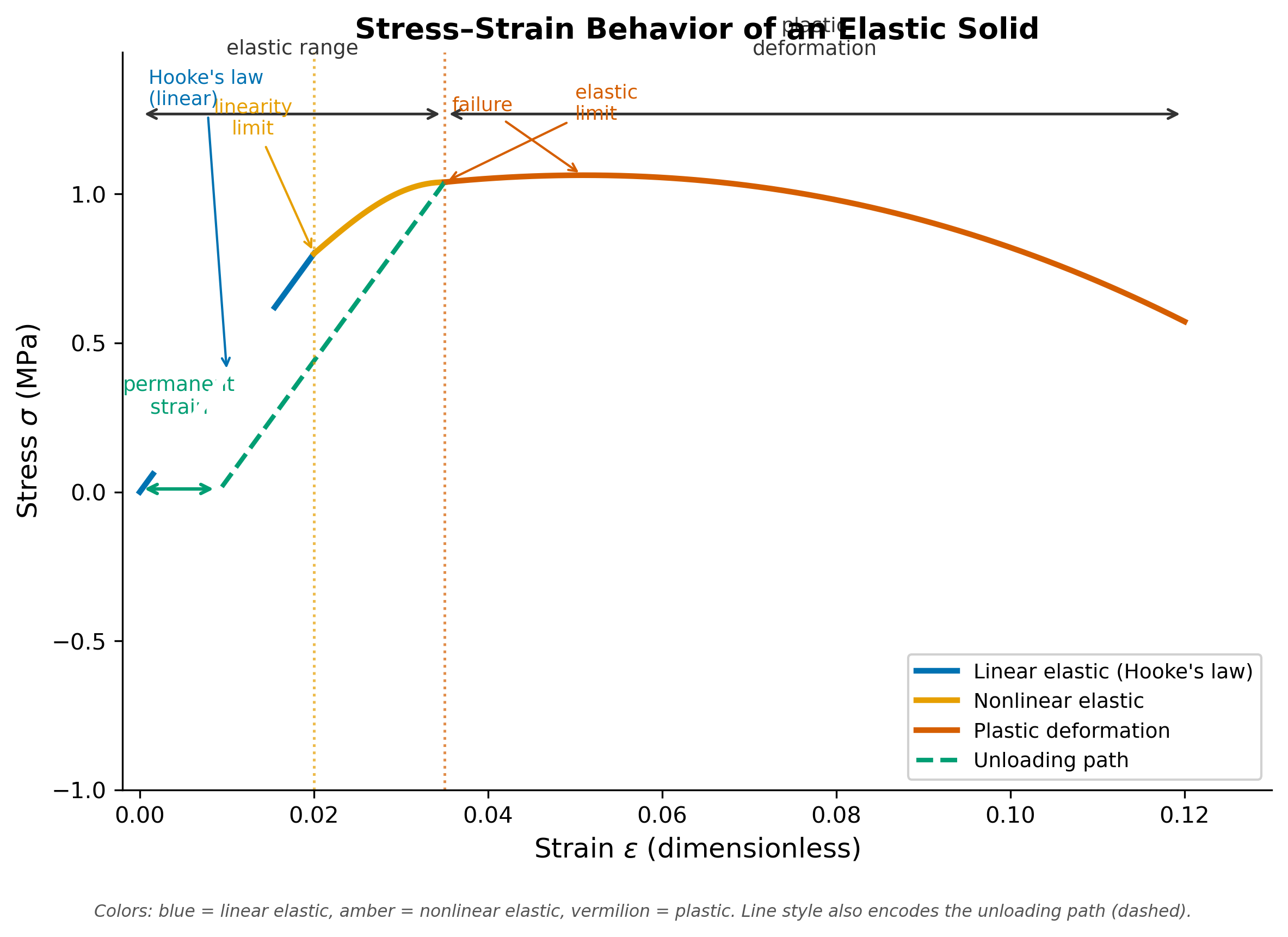
Stress-strain curve showing four regions: a blue linear elastic zone labeled Hooke's law where stress is proportional to strain, an amber nonlinear elastic zone, an orange plastic deformation zone, and a dashed green unloading path showing permanent strain. Vertical dashed lines mark the linearity limit and elastic limit. — Fig. 4 **Figure 3.1.** Stress–strain behavior of an elastic solid. Seismic waves operate entirely in the blue (Hookean) region. The elastic limit and plastic zone are relevant to fault mechanics and rock failure, not wave propagation. [Python-generated. Script: `assets/scripts/fig_stress_strain_curve.py`]#

2.2 Two Fundamental Modes of Elastic Deformation#

Any deformation of an isotropic solid can be decomposed into two orthogonal modes:

Volumetric strain (dilatation, $\theta$): a fractional change in volume with no change in shape. A cube compressed equally on all sides shrinks without becoming a non-cube. This mode requires a resistance to volume change, characterized by the bulk modulus $K$.

Shear strain ($\varepsilon_{ij}$, $i \neq j$): a change in shape with no change in volume. A cube distorts into a parallelepiped. This mode requires a resistance to shape change, characterized by the shear modulus $\mu$.

This decomposition is not merely convenient — it directly maps onto the two fundamental seismic wave types: P-waves involve volumetric strain; S-waves involve shear strain only.

3. Mathematical Framework#

3.1 The Stress Tensor#

Notation

Symbol	Quantity	Units	Type
$\mathbf{F}$	Force vector	N	vector
$A$	Surface area	m²	scalar
$\sigma_{ij}$	Stress component: force per unit area in $i$-direction on surface with outward normal in $j$-direction	Pa	tensor component
$\boldsymbol{\sigma}$	Stress tensor	Pa	2nd-order symmetric tensor
$\varepsilon_{ij}$	Strain component	dimensionless	tensor component
$\boldsymbol{\varepsilon}$	Strain tensor	—	2nd-order symmetric tensor
$u_i$	Displacement component in direction $i$	m	vector component
$\mathbf{u}$	Displacement vector	m	vector
$\theta$	Dilatation (volumetric strain) $= \nabla \cdot \mathbf{u}$	dimensionless	scalar
$\delta_{ij}$	Kronecker delta ($=1$ if $i=j$, else $0$)	—	—
$E$	Young’s modulus	Pa	scalar
$K$	Bulk modulus	Pa	scalar
$\mu$	Shear modulus (rigidity)	Pa	scalar
$\nu$	Poisson’s ratio	dimensionless	scalar
$\lambda$	First Lamé parameter	Pa	scalar
$\rho$	Density	kg/m³	scalar

Stress is force per unit area. In 3D, specifying the stress state at a point requires knowing the force components on three independent surfaces, yielding nine numbers organized as the stress tensor:

(1)#\[\begin{split} \boldsymbol{\sigma} = \begin{pmatrix} \sigma_{xx} & \sigma_{xy} & \sigma_{xz} \\ \sigma_{yx} & \sigma_{yy} & \sigma_{yz} \\ \sigma_{zx} & \sigma_{zy} & \sigma_{zz} \end{pmatrix} \end{split}\]

The diagonal components are normal stresses (compression/tension perpendicular to a face). The off-diagonal components are shear stresses (forces parallel to a face). By conservation of angular momentum — requiring that the stress state produces no net torque on a small element — the tensor is symmetric:

(2)#\[ \sigma_{ij} = \sigma_{ji} \]

Symmetry reduces the 9 independent components to 6.

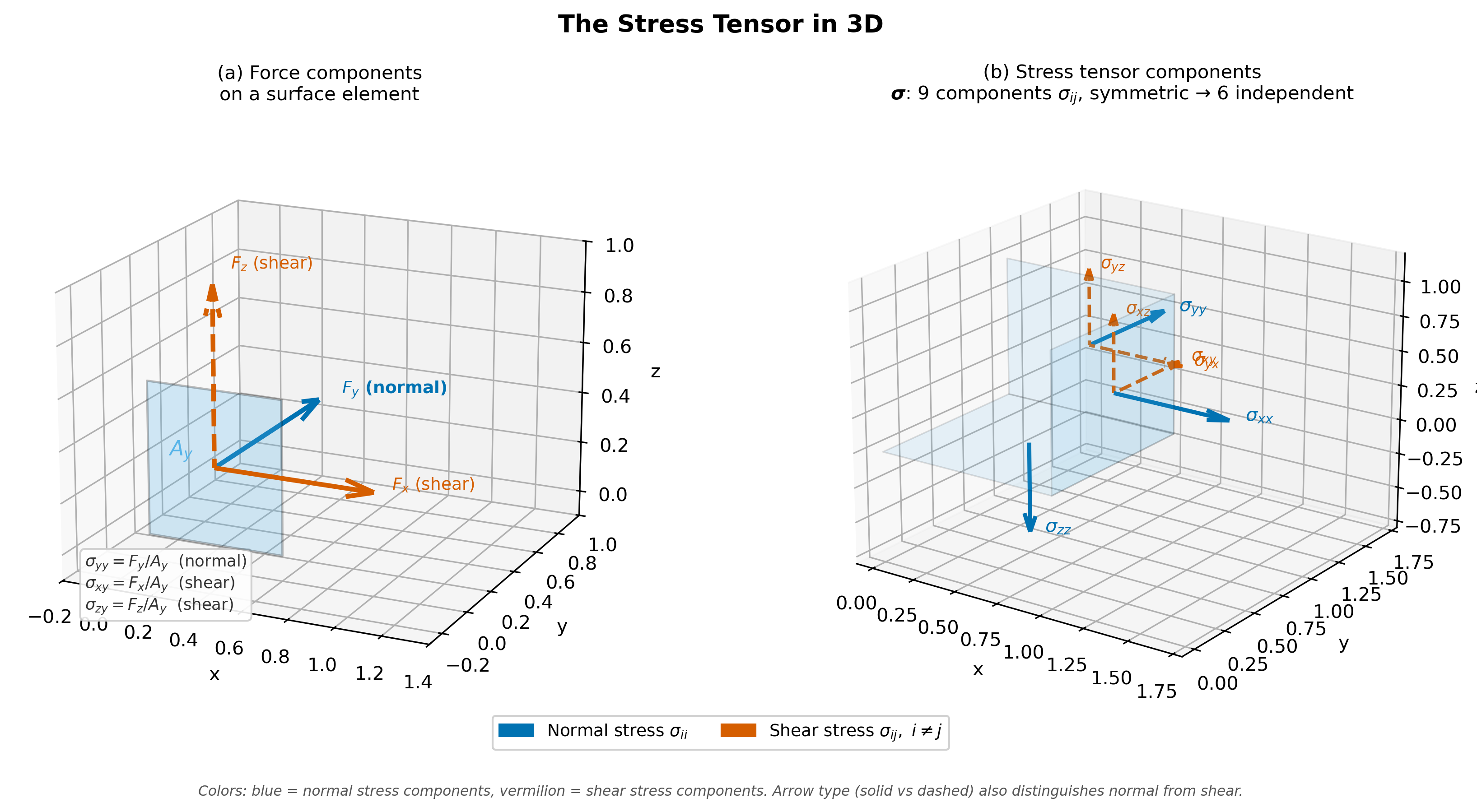
Two 3D diagrams. Left panel shows a surface element with one normal force and two shear forces labeled with component notation. Right panel shows a unit cube with six distinct stress components as arrows on the three visible faces, colored blue for normal stresses and vermilion for shear stresses. — Fig. 5 **Figure 3.2.** The stress tensor in 3D. Left: three independent force components act on any surface element. Right: the full tensor on a unit cube — 9 components reduced to 6 by symmetry $\sigma_{ij} = \sigma_{ji}$. [Python-generated. Script: `assets/scripts/fig_stress_tensor.py`]#

3.2 The Strain Tensor#

Strain measures how a material deforms relative to its original state. Consider two material points initially at positions $x$ and $x + \Delta x$. Under deformation, they displace by $u(x)$ and $u(x+\Delta x) = u(x) + (\partial u/\partial x)\Delta x$. The fractional change in their separation — the longitudinal strain — is:

(3)#\[ \varepsilon_{xx} = \frac{\partial u_x}{\partial x} \]

Units check: [m/m] = dimensionless ✓

In 3D, stretches occur independently in all three directions, and the material can also shear. The shear strain component $\varepsilon_{xy}$ measures the average angular distortion of a right angle originally aligned with the $x$–$y$ axes:

(4)#\[ \varepsilon_{xy} = \frac{1}{2}\left(\frac{\partial u_x}{\partial y} + \frac{\partial u_y}{\partial x}\right) \]

The factor of $\frac{1}{2}$ isolates pure deformation from rigid-body rotation: a pure rotation has $\partial u_x/\partial y = -\partial u_y/\partial x$, giving $\varepsilon_{xy} = 0$ — correct, since rigid rotation is not deformation.

The complete strain tensor in compact notation is:

(5)#\[ \varepsilon_{ij} = \frac{1}{2}\left(\frac{\partial u_i}{\partial x_j} + \frac{\partial u_j}{\partial x_i}\right) \]

Key Equation: Strain Tensor

Equation (5) is the symmetric part of the displacement gradient tensor. It has six independent components (like the stress tensor) and automatically excludes rigid-body rotation. The diagonal components measure extension/compression; the off-diagonal components measure angular distortion.

The dilatation — fractional volume change — is the trace:

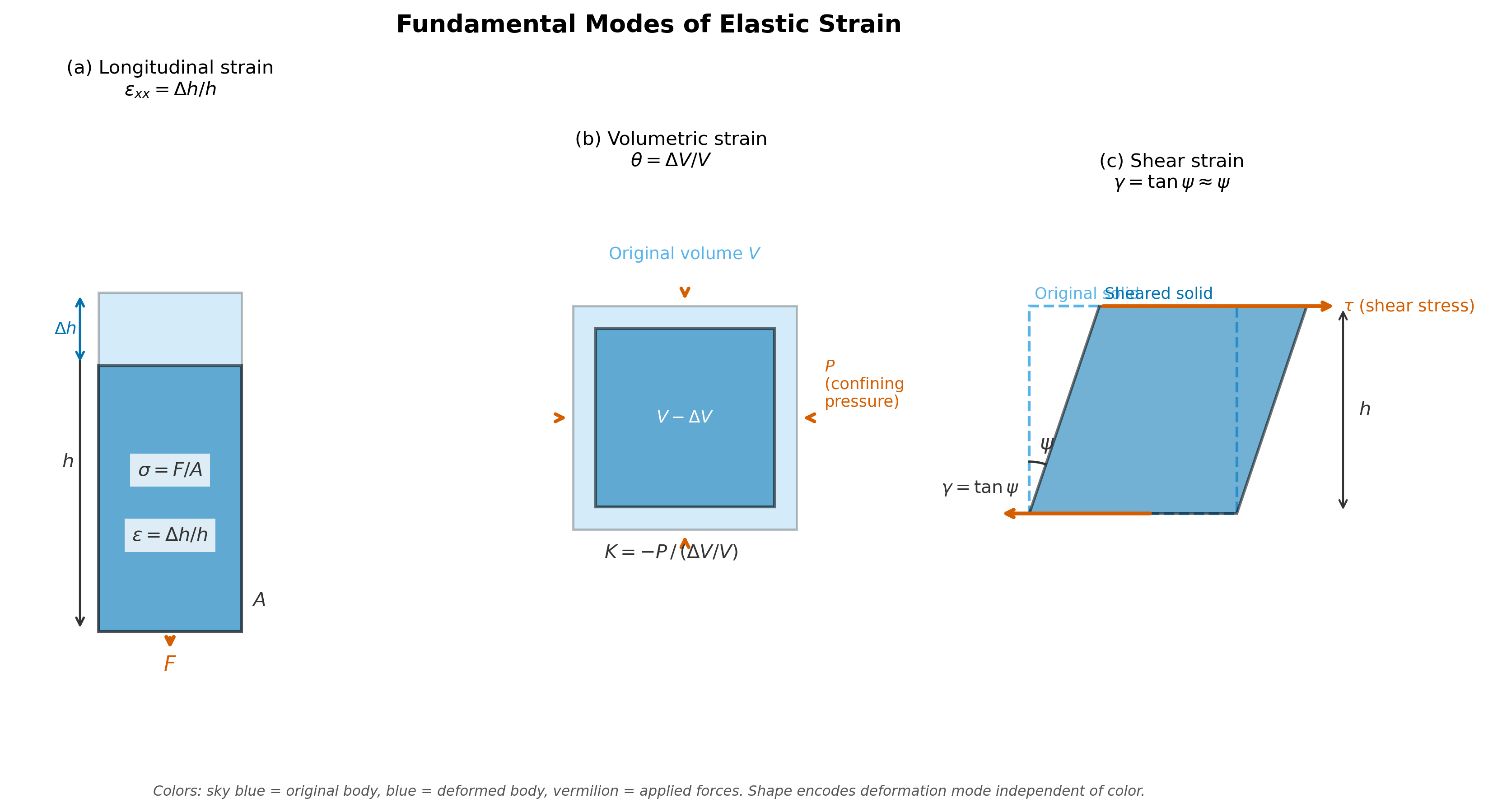
(6)#\[ \theta = \varepsilon_{xx} + \varepsilon_{yy} + \varepsilon_{zz} = \nabla \cdot \mathbf{u} \]

Three-panel figure showing longitudinal strain as a cylinder compressed axially with dimension labels, volumetric strain as a cube compressed uniformly with four pressure arrows, and shear strain as a rectangle distorted into a parallelogram with an angle psi labeled at the corner. — Fig. 6 **Figure 3.3.** The three fundamental modes of strain. (a) Longitudinal: $\varepsilon_{xx} = \partial u_x / \partial x$. (b) Volumetric (dilatation): $\theta = \nabla \cdot \mathbf{u}$. (c) Shear: $\varepsilon_{xy} = \frac{1}{2}(\partial u_x/\partial y + \partial u_y/\partial x)$. [Python-generated. Script: `assets/scripts/fig_strain_types.py`]#

3.3 Elastic Moduli: Four Ways to Resist Deformation#

Elastic moduli quantify how strongly a material resists each mode of deformation. For an isotropic solid, four independent moduli are in common use; any two of them fully specify the elastic behavior.

Four-panel figure. Panel 1 shows Young's modulus with a tall blue rectangle compressed vertically to a shorter rectangle by a downward force, with the equation E equals sigma over epsilon. Panel 2 shows shear modulus with a rectangle sheared into a parallelogram by a horizontal force, with angle theta and equation mu equals tau over gamma. Panel 3 shows bulk modulus with a cube compressed from all sides by confining pressure P arrows, with equation K equals negative P divided by delta-V over V. Panel 4 shows Poisson ratio with a cylinder compressed axially that bulges laterally, with equation nu equals negative lateral strain divided by axial strain. 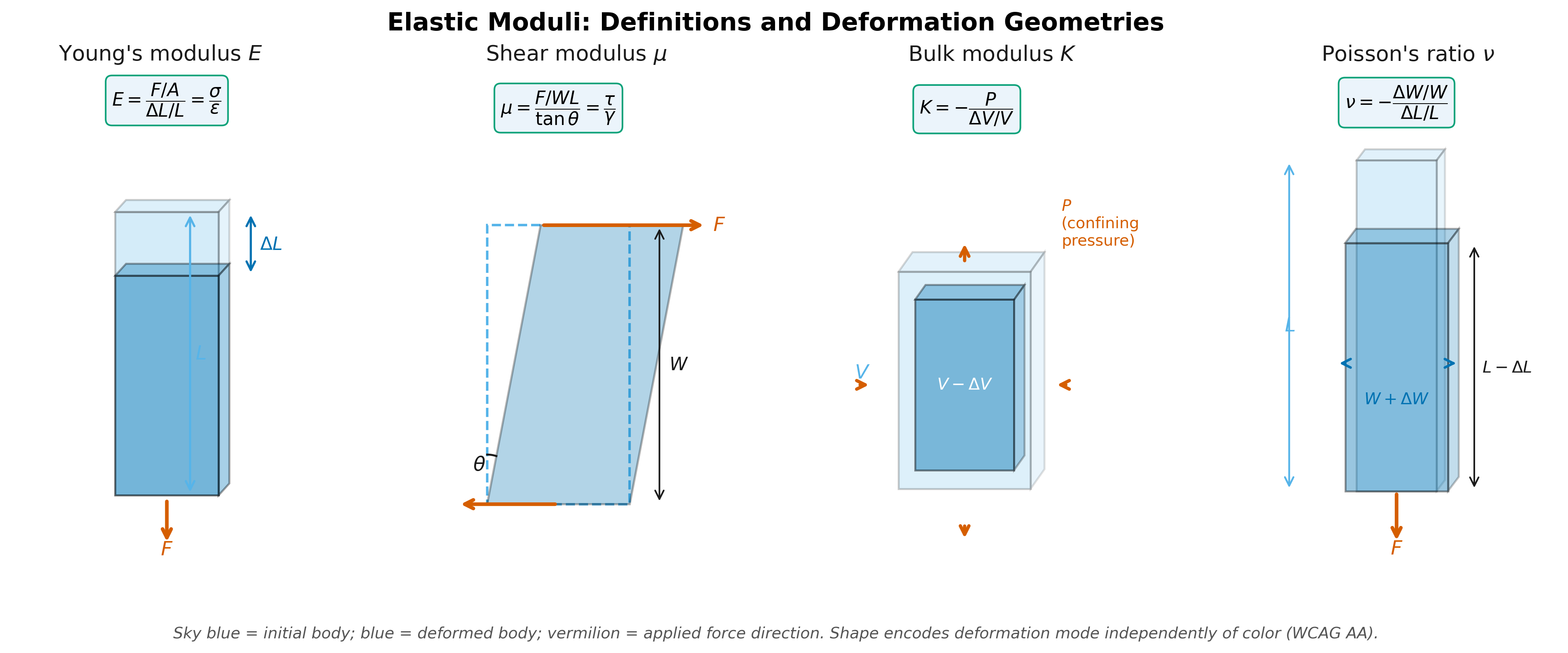— Fig. 7 **Figure 3.4.** The four principal elastic moduli: Young’s modulus $E$ (axial stiffness), shear modulus $\mu$ (shear stiffness), bulk modulus $K$ (resistance to volume change), and Poisson’s ratio $\nu$ (lateral-to-axial strain ratio). [Python-generated. Script: `assets/scripts/fig_elastic_moduli.py`]#

Young’s modulus $E$ relates uniaxial stress to uniaxial strain in a slender rod:

(7)#\[ E = \frac{\sigma_{xx}}{\varepsilon_{xx}}\bigg|_\text{uniaxial} \]

Bulk modulus $K$ relates hydrostatic pressure to volumetric strain:

(8)#\[ K = -\frac{P}{\Delta V / V} = -\frac{P}{\theta} \]

Shear modulus $\mu$ relates shear stress to shear strain:

(9)#\[ \mu = \frac{\tau}{\gamma} = \frac{\sigma_{xy}}{\varepsilon_{xy}} \]

Poisson’s ratio $\nu$ is the ratio of lateral to axial strain under uniaxial stress:

(10)#\[ \nu = -\frac{\varepsilon_{yy}}{\varepsilon_{xx}}\bigg|_\text{uniaxial} \]

Typical values for crustal rocks: $0.20 \lesssim \nu \lesssim 0.35$, with most igneous rocks near $0.25$–$0.30$. Saturated sediments and fluids approach $\nu = 0.5$ (perfectly incompressible — no resistance to shear, maximum lateral expansion under axial load). These four moduli are related — any two fix all others. The pair most natural for seismology is the Lamé parameters $\lambda$ and $\mu$:

(11)#\[ \lambda = \frac{\nu E}{(1+\nu)(1-2\nu)} = K - \frac{2\mu}{3}, \qquad \mu = \frac{E}{2(1+\nu)} \]

The Lamé parameters appear directly in the most general form of Hooke’s law, which is why seismologists prefer them.

3.4 Isotropic Hooke’s Law#

For a homogeneous, isotropic, linear elastic solid, the stress tensor is related to the strain tensor by:

(12)#\[ \sigma_{ij} = \lambda\,\delta_{ij}\,\theta + 2\mu\,\varepsilon_{ij} \]

Units check: $[\lambda][\theta] = \text{Pa} \cdot \text{dimensionless} = \text{Pa}$. $[\mu][\varepsilon_{ij}] = \text{Pa}$. Sum gives Pa = $[\sigma_{ij}]$ ✓

Key Equation: Isotropic Hooke’s Law

\[ \sigma_{ij} = \lambda\,\delta_{ij}\,\theta + 2\mu\,\varepsilon_{ij} \]

Physical interpretation:

The first term $\lambda\,\delta_{ij}\,\theta$ acts only on the diagonal (normal stresses) and couples all three axial directions through the dilatation $\theta = \varepsilon_{kk}$. It represents the contribution of volume change to normal stress.
The second term $2\mu\,\varepsilon_{ij}$ affects all components (both normal and shear). It represents the direct resistance to any strain.
Why only two parameters? For an isotropic solid, all directions are equivalent, so the stiffness tensor — which in general has 21 independent components — collapses to just 2.

Writing out the $xx$-component explicitly:

(13)#\[ \sigma_{xx} = \lambda\,\theta + 2\mu\,\varepsilon_{xx} = \lambda(\varepsilon_{xx}+\varepsilon_{yy}+\varepsilon_{zz}) + 2\mu\,\varepsilon_{xx} \]

Even if there is no strain in $x$ ($\varepsilon_{xx} = 0$), compression in $y$ and $z$ still generates a normal stress in $x$ through $\lambda$. This coupling between deformation modes is what distinguishes 3D elastic behavior from a simple spring.

3.5 The Force Balance: Deriving the Equation of Motion#

Now combine the stress tensor with Newton’s second law to find how stress gradients drive particle acceleration. Consider an infinitesimal element between positions $x$ and $x + dx$, with cross-sectional area $A_x$ and density $\rho$.

Two-panel figure. Left panel shows a thin elastic element between x and x plus dx with face area labeled A_x and two displacement arrows labeled u at x and u plus du at x plus dx. Right panel shows the same element with a vermilion force arrow F_x entering from the left face and a larger F_x plus dF_x arrow leaving the right face, with equation boxes showing the net force, Newton's second law, and the final equation of motion rho times second partial of u over t-squared equals partial of sigma-xx over x. 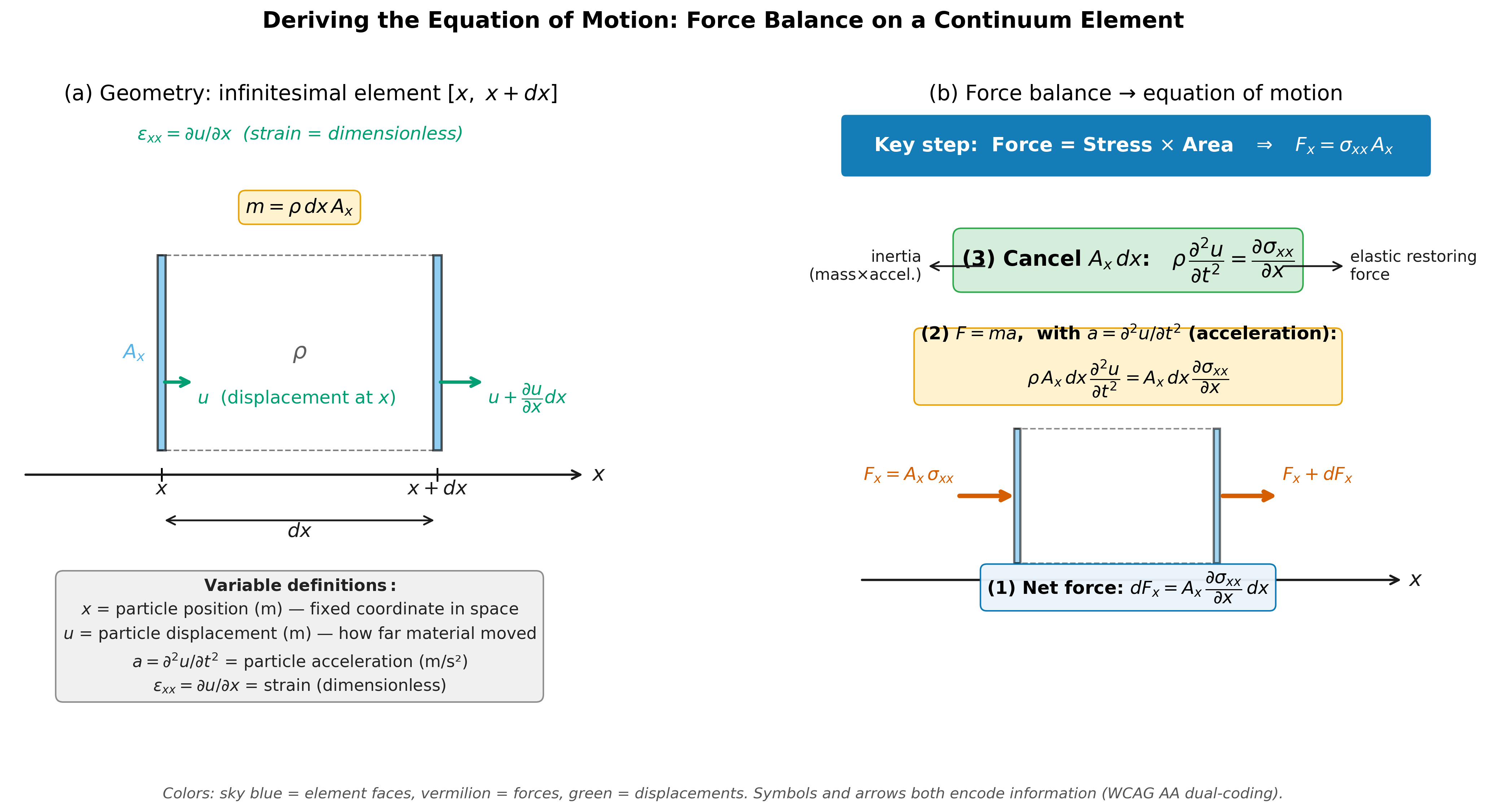— Fig. 8 **Figure 3.5.** Force balance on an infinitesimal continuum element. The net force (difference between stresses on the two faces) equals mass times acceleration. [Python-generated. Script: `assets/scripts/fig_force_balance.py`]#

Step 1 — Mass of the element:

(14)#\[ m = \rho\,A_x\,dx \]

Step 2 — Forces on the element. The normal stress on the left face is $\sigma_{xx}(x)$; the force is $F_x = A_x\,\sigma_{xx}$. On the right face, the stress has changed by $(\partial\sigma_{xx}/\partial x)dx$, so the force is $F_x + dF_x = A_x[\sigma_{xx} + (\partial\sigma_{xx}/\partial x)dx]$. The net force in the $x$-direction:

(15)#\[ dF_x = A_x\,\frac{\partial\sigma_{xx}}{\partial x}\,dx \]

Step 3 — Newton’s second law $\sum F = ma$ with $a = \partial^2 u/\partial t^2$:

\[ A_x\,\frac{\partial\sigma_{xx}}{\partial x}\,dx = \rho\,A_x\,dx\,\frac{\partial^2 u}{\partial t^2} \]

Cancel $A_x\,dx$ (non-zero):

(16)#\[ \rho\,\frac{\partial^2 u}{\partial t^2} = \frac{\partial\sigma_{xx}}{\partial x} \]

Step 4 — Substitute Hooke’s law. For a longitudinal (P-type) wave propagating in $x$, the relevant strain is $\varepsilon_{xx} = \partial u/\partial x$, and the 1D form of Hooke’s law gives $\sigma_{xx} = (\lambda + 2\mu)\,\varepsilon_{xx}$. Therefore:

\[ \frac{\partial\sigma_{xx}}{\partial x} = (\lambda + 2\mu)\,\frac{\partial^2 u}{\partial x^2} \]

Substituting into (16):

(17)#\[ \rho\,\frac{\partial^2 u}{\partial t^2} = (\lambda + 2\mu)\,\frac{\partial^2 u}{\partial x^2} \]

Key Equation: 1D P-wave Equation

\[ \rho\,\frac{\partial^2 u}{\partial t^2} = (\lambda + 2\mu)\,\frac{\partial^2 u}{\partial x^2} \]

This is a wave equation of the standard form $\partial^2 u/\partial t^2 = V^2\,\partial^2 u/\partial x^2$ with:

(18)#\[ V_P = \sqrt{\frac{\lambda + 2\mu}{\rho}} \]

Left side: Inertia — how much mass resists acceleration. Right side: Elastic restoring force — how strongly the medium resists strain. Their ratio fixes the wave speed. A stiffer medium ($\lambda + 2\mu$ large) propagates waves faster. A denser medium ($\rho$ large) propagates waves more slowly.

Units: $[V_P] = \sqrt{\text{Pa}/(\text{kg/m}^3)} = \sqrt{(\text{kg}\,\text{m}^{-1}\,\text{s}^{-2})/(\text{kg}\,\text{m}^{-3})} = \sqrt{\text{m}^2\,\text{s}^{-2}} = \text{m/s}$ ✓

The same derivation for shear motion (transverse displacement, strain $\varepsilon_{xy}$, stress $\sigma_{xy} = \mu\,\varepsilon_{xy}$) yields:

(19)#\[ \rho\,\frac{\partial^2 u}{\partial t^2} = \mu\,\frac{\partial^2 u}{\partial x^2} \qquad\Rightarrow\qquad V_S = \sqrt{\frac{\mu}{\rho}} \]

Since $\lambda \geq 0$ for any stable elastic material, $\lambda + 2\mu > \mu$, and therefore $V_P > V_S$ — always. The P-wave always arrives before the S-wave.

3.6 Extending to Three Dimensions: The Vector Equation of Motion#

The 1D derivation above is sufficient to introduce wave speeds, but it only captures motion along a single axis. A real earthquake radiates energy in all directions, and the displacement field $\mathbf{u}(\mathbf{x},t)$ is a full 3D vector field. To describe it, we repeat the force-balance argument on all six faces of an infinitesimal 3D element.

Step 1 — Generalize the force balance to 3D. In 3D, the stress on each pair of faces contributes to the net force. The net force per unit volume in direction $i$ from all stress gradients is:

(20)#\[ f_i = \frac{\partial \sigma_{i1}}{\partial x_1} + \frac{\partial \sigma_{i2}}{\partial x_2} + \frac{\partial \sigma_{i3}}{\partial x_3} = \frac{\partial \sigma_{ij}}{\partial x_j} \]

where the repeated index $j$ is summed (Einstein summation convention). Combining with Newton’s second law gives the Cauchy equation of motion:

(21)#\[ \rho\,\frac{\partial^2 u_i}{\partial t^2} = \frac{\partial \sigma_{ij}}{\partial x_j} \]

Units check: $[\rho]\,[u/t^2] = (\text{kg/m}^3)(\text{m/s}^2) = \text{kg/(m}^2\text{s}^2) = \text{Pa/m}$. Right side: $[\sigma_{ij}/x_j] = \text{Pa/m}$ ✓

Step 2 — Substitute Hooke’s law. Insert $\sigma_{ij} = \lambda\,\delta_{ij}\,\theta + 2\mu\,\varepsilon_{ij}$ from (12) into (21). For a homogeneous medium ($\lambda$, $\mu$ spatially constant):

(22)#\[ \frac{\partial \sigma_{ij}}{\partial x_j} = \lambda\,\delta_{ij}\,\frac{\partial \theta}{\partial x_j} + 2\mu\,\frac{\partial \varepsilon_{ij}}{\partial x_j} = \lambda\,\frac{\partial \theta}{\partial x_i} + 2\mu\,\frac{\partial \varepsilon_{ij}}{\partial x_j} \]

The $\delta_{ij}$ collapses the sum to a single term: $\delta_{ij}\partial\theta/\partial x_j = \partial\theta/\partial x_i$. Now expand the strain divergence using (5):

(23)#\[ \frac{\partial \varepsilon_{ij}}{\partial x_j} = \frac{1}{2}\frac{\partial}{\partial x_j}\!\left(\frac{\partial u_i}{\partial x_j} + \frac{\partial u_j}{\partial x_i}\right) = \frac{1}{2}\frac{\partial^2 u_i}{\partial x_j^2} + \frac{1}{2}\frac{\partial}{\partial x_i}\!\underbrace{\left(\frac{\partial u_j}{\partial x_j}\right)}_{=\,\theta} = \frac{1}{2}\nabla^2 u_i + \frac{1}{2}\frac{\partial \theta}{\partial x_i} \]

Step 3 — Assemble the Navier equation. Substituting (23) into (22) and writing in vector form:

(24)#\[ \rho\,\frac{\partial^2\mathbf{u}}{\partial t^2} = (\lambda + \mu)\,\nabla(\nabla\cdot\mathbf{u}) + \mu\,\nabla^2\mathbf{u} \]

This is the Navier–Cauchy equation of linear elasticity. It governs the displacement field in any homogeneous, isotropic, linearly elastic solid.

Step 4 — Apply a vector identity. The vector Laplacian satisfies the identity:

(25)#\[ \nabla^2\mathbf{u} = \nabla(\nabla\cdot\mathbf{u}) - \nabla\times(\nabla\times\mathbf{u}) \]

Substituting (25) into (24):

\[ \rho\,\frac{\partial^2\mathbf{u}}{\partial t^2} = (\lambda+\mu)\,\nabla(\nabla\cdot\mathbf{u}) + \mu\bigl[\nabla(\nabla\cdot\mathbf{u}) - \nabla\times(\nabla\times\mathbf{u})\bigr] \]

Collecting the $\nabla(\nabla\cdot\mathbf{u})$ terms yields the canonical form:

(26)#\[ \rho\,\frac{\partial^2\mathbf{u}}{\partial t^2} = (\lambda+2\mu)\,\nabla(\nabla\cdot\mathbf{u}) - \mu\,\nabla\times(\nabla\times\mathbf{u}) \]

Key Equation: 3D Vector Equation of Motion

\[ \rho\,\frac{\partial^2\mathbf{u}}{\partial t^2} = (\lambda+2\mu)\,\nabla(\nabla\cdot\mathbf{u}) - \mu\,\nabla\times(\nabla\times\mathbf{u}) \]

Physical interpretation of the two terms:

Term	Operator	What it measures	Elastic resistance	Wave type
$(\lambda+2\mu)\,\nabla(\nabla\cdot\mathbf{u})$	$\nabla(\nabla\cdot)$	Gradient of dilatation $\theta = \nabla\cdot\mathbf{u}$ — where volume is changing	$\lambda+2\mu = K + \tfrac{4}{3}\mu$ (bulk + shear)	P-wave
$-\mu\,\nabla\times(\nabla\times\mathbf{u})$	$\nabla\times(\nabla\times)$	Curl of rotation — where the medium is spinning	$\mu$ (shear only)	S-wave

The equation encodes the same physics as the two 1D equations in §3.5, but in a single vector statement that is direction-independent and valid for waves traveling in any direction through any isotropic solid.

Consistency check: recovery of the 1D results. Let $\mathbf{u} = u(x,t)\,\hat{\mathbf{x}}$ — displacement only in $x$, varying only with $x$. Then:

\[ \nabla\cdot\mathbf{u} = \frac{\partial u}{\partial x}, \qquad \nabla\times\mathbf{u} = \mathbf{0}. \]

Equation (26) becomes:

\[ \rho\,\frac{\partial^2 u}{\partial t^2} = (\lambda+2\mu)\,\frac{\partial^2 u}{\partial x^2} \]

— exactly the P-wave equation (17) from §3.5. ✓

For a transverse displacement $\mathbf{u} = u(x,t)\,\hat{\mathbf{z}}$, we have $\nabla\cdot\mathbf{u} = 0$ and $\nabla\times(\nabla\times\mathbf{u}) = -(\partial^2 u/\partial x^2)\,\hat{\mathbf{z}}$, recovering the S-wave equation (32). ✓

Look Ahead — Lecture 4

Equation (26) has a remarkable property: in a homogeneous medium, its right-hand side separates into two non-interacting terms. In Lecture 4, we will formalize this using the Helmholtz decomposition, writing $\mathbf{u} = \nabla\phi + \nabla\times\boldsymbol{\psi}$. Substituting shows that $\phi$ satisfies a scalar wave equation at speed $V_P$ and $\boldsymbol{\psi}$ satisfies a vector wave equation at speed $V_S$ — independently. The same elastic wave equation spawns two distinct wave families, each carrying different information about the subsurface.

4. The Forward Problem#

Given the elastic properties of a rock column — $\lambda(z)$, $\mu(z)$, $\rho(z)$ as functions of depth — the forward problem predicts:

Model parameters: $\lambda(z)$, $\mu(z)$, $\rho(z)$

Observables predicted:

$V_P(z) = \sqrt{(\lambda + 2\mu)/\rho}$ at each depth
$V_S(z) = \sqrt{\mu/\rho}$ at each depth
Travel time for a wave from source to receiver at distance $\Delta$
The waveform recorded at a seismometer

See companion notebook: notebooks/lecture_03_wave_speeds.ipynb

Worked Example — Crustal Rock:

A granitic rock has $\lambda = 30$ GPa, $\mu = 25$ GPa, $\rho = 2700$ kg/m³.

\[ V_P = \sqrt{\frac{30 + 2 \times 25}{2700} \times 10^9} = \sqrt{\frac{80 \times 10^9}{2700}} = \sqrt{2.963 \times 10^7} \approx 5443 \text{ m/s} \]

\[ V_S = \sqrt{\frac{25 \times 10^9}{2700}} = \sqrt{9.26 \times 10^6} \approx 3043 \text{ m/s} \]

\[ \frac{V_P}{V_S} = \sqrt{\frac{\lambda + 2\mu}{\mu}} = \sqrt{\frac{80}{25}} = \sqrt{3.2} \approx 1.79 \]

Using $\nu = \lambda / [2(\lambda + \mu)]$:

\[ \nu = \frac{30}{2 \times (30 + 25)} = \frac{30}{110} \approx 0.27 \]

This is characteristic of upper-crustal granite.

5. The Inverse Problem#

Inverse Problem Setup

Data $d$: Seismic wave travel times recorded at seismometers
Model $m$: Elastic properties $\lambda(z)$, $\mu(z)$, $\rho(z)$ as functions of depth
Forward relation: $d = G(m)$ where $G$ computes travel times from the velocity model via $V_P = \sqrt{(\lambda+2\mu)/\rho}$
Key non-uniqueness: Travel times alone cannot separately constrain $\lambda$, $\mu$, and $\rho$ — only the combinations $V_P$ and $V_S$. Density requires independent amplitude or gravity information.
Resolution limit: Only velocity structure at scales larger than the dominant wavelength $\lambda_\text{dom} = V/f$ is recoverable.

Note the index mismatch that always requires care: the Lamé parameter $\lambda$ appears both in Hooke’s law and loosely in the notation $\lambda_\text{dom}$ for wavelength. The convention in this course: $\lambda$ (roman, upright) is Lamé’s first parameter; wavelength will always be written out or subscripted.

6. Worked Example: $V_P/V_S$ as a Fluid Diagnostic#

Sediment at a borehole site: measured $V_P = 1800$ m/s and $V_S = 300$ m/s.

The $V_P/V_S$ ratio: $$ \frac{V_P}{V_S} = \frac{1800}{300} = 6.0 $$

Poisson’s ratio from velocities: $$ \nu = \frac{V_P^2 - 2V_S^2}{2(V_P^2 - V_S^2)} = \frac{1800^2 - 2 \times 300^2}{2(1800^2 - 300^2)} = \frac{3{,}240{,}000 - 180{,}000}{2(3{,}240{,}000 - 90{,}000)} = \frac{3{,}060{,}000}{6{,}300{,}000} \approx 0.486 $$

This $\nu \approx 0.49$ is close to the incompressible fluid limit of 0.5. The interpretation: these sediments are water-saturated, and their $V_P$ is controlled primarily by the pore fluid (water at ~1500 m/s), while $V_S$ is low because the unconsolidated sediment matrix has very little shear rigidity. This condition — high $V_P/V_S$ in soft near-surface sediment — is exactly what causes earthquake ground motions to be amplified in Seattle’s Pioneer Square district relative to adjacent bedrock sites.

Concept Check

A rock sample has $E = 70$ GPa and $\nu = 0.28$. Calculate $\mu$, $K$, $\lambda$, $V_P$, and $V_S$ assuming $\rho = 2850$ kg/m³. Show all unit checks.
A sediment layer has $V_P = 1500$ m/s but $V_S = 50$ m/s. What does this imply about its Poisson’s ratio and physical state? Is this physically plausible? (Hint: consider what happens to $K$ and $\mu$ in a fluid-saturated sediment.)
The equation $V_P = \sqrt{E/\rho}$ is sometimes quoted for P-waves. Under what specific conditions is this correct, and how does it differ from $V_P = \sqrt{(\lambda+2\mu)/\rho}$? (Hint: think about boundary conditions — constrained vs. unconstrained lateral deformation.)

7. Course Connections#

Prior lectures: This lecture applies the force-per-unit-area definition of stress from Lecture 2, extends it to a 3D tensor, and introduces strain as the kinematic complement. Lecture 3 is the bridge from statics (Lecture 2) to dynamics (Lectures 4–6).
Next lecture (Lecture 4): Seismic wave types — P, S, Rayleigh, Love — and the Helmholtz decomposition that separates the vector equation of motion (26) into two independent wave families. The $\nabla(\nabla\cdot\mathbf{u})$ term derived in §3.6 will be identified as the P-wave driver; the $\nabla\times(\nabla\times\mathbf{u})$ term as the S-wave driver. We will use $V_P$ and $V_S$ from this lecture as the two wave speeds throughout.
Lecture 5: Reflection and refraction seismology — the travel-time equations all descend from the wave equation derived here.
Lab 2: Students will write Python code to compute $V_P$, $V_S$, and $V_P/V_S$ as functions of depth for a layered crustal model, then plot the results and interpret them.
Cross-topic: The elastic moduli derived here reappear in every geophysical method. In gravity, density $\rho$ is the primary observable. In magnetics, rock composition (which determines both magnetic properties and moduli) provides joint constraints. The $V_P/V_S$ ratio is arguably the single most useful diagnostic in applied seismology.

8. Research Horizon#

Current Research Highlights (2022–2025)

Machine learning inversion of elastic moduli. Classical inversion of seismic velocities for $\lambda$, $\mu$, and $\rho$ separately requires combining P-wave and S-wave traveltimes with amplitude information, and the problem is strongly non-unique. Physics-informed neural networks (PINNs) are being used to jointly invert these properties by embedding the wave equation as a constraint in the loss function, allowing the network to enforce physical consistency rather than treating the problem as unconstrained regression. Several 2023–2024 papers demonstrate PINN-based inversion on synthetic and real seismic datasets (see Rasht-Behesht et al., 2022, JGR Solid Earth, doi:10.1029/2021JB023120).

Elastic anisotropy at depth. The derivation in this lecture assumed isotropy — elastic properties the same in all directions. Real rocks are often anisotropic: olivine crystals in the mantle align under flow, creating directionally dependent wave speeds. Measuring this anisotropy with seismic shear-wave splitting is an active area for constraining mantle flow directions. New waveform modeling tools treat the full anisotropic stiffness tensor (21 independent components instead of 2), which requires everything developed in this lecture plus tensorial generalizations (see Bodin et al., 2023, Annual Review of Earth and Planetary Sciences, doi:10.1146/annurev-earth-071522-122118 (⚠ DOI returns 404 — verify manually)).

Non-destructive testing via elastic wave imaging. The same equations that govern earthquake wave propagation apply at laboratory scale: ultrasonic P-wave and S-wave speeds in rock cores directly yield $\lambda$, $\mu$, and $\nu$ from (31) and (32). Laboratories at EarthScope and UNAVCO provide standardized equipment for this, and the data feed into global databases of rock elastic properties used to calibrate seismic Earth models.

DAS-based surface wave monitoring of elastic structure. Distributed Acoustic Sensing (DAS) converts existing fiber-optic cables into dense seismic arrays with sensor spacing of a few meters, enabling retrieval of Rayleigh-wave dispersion curves along thousands of channels simultaneously. Viens et al. (2023, Geophysical Journal International, doi:10.1093/gji/ggad186 (⚠ DOI resolves to a different paper — verify manually)) showed that ambient-noise Rayleigh wave analysis on urban DAS arrays recovers near-surface $V_S$ profiles at centimeter-scale resolution — the same $\mu/\rho$ relationship derived in this lecture. Fukushima et al. (2024, GJI, doi:10.1093/gji/ggae103) extended this approach to submarine fiber cables, opening a path to monitoring elastic properties beneath the ocean floor.

For students interested in this area: The IRIS SSBW (Seismology Skill Building Workshop) covers hands-on velocity inversion with ObsPy each summer — a natural entry point using the physics from today’s lecture. See iris.edu/hq/workshops.

9. Societal Relevance#

Why It Matters: Ground Motion Amplification in Seattle

The Seattle Basin amplification problem. Seattle sits above a deep sedimentary basin — the Seattle Basin — where soft water-saturated sediments with $V_S$ as low as 150–400 m/s overlie bedrock with $V_S > 3000$ m/s. The equations in this lecture explain why this is dangerous: seismic energy is conserved as waves cross the velocity contrast, so the amplitude must increase when the wave slows down (by roughly the square root of the impedance ratio $\rho_\text{bedrock} V_{S,\text{bedrock}} / \rho_\text{sed} V_{S,\text{sed}}$). This can amplify shaking by factors of 5–10 in the basin relative to adjacent rock sites.

The 2001 Nisqually earthquake (M 6.8) demonstrated this dramatically: damage in Seattle’s Pioneer Square district on thick sediments was disproportionately severe compared to Capitol Hill or Queen Anne on till. The current USGS probabilistic seismic hazard models for the Pacific Northwest incorporate site-amplification factors derived precisely from the velocity contrasts ($V_P$, $V_S$) you calculated in this lecture.

For further exploration:

USGS Earthquake Hazards Program, Seattle Basin amplification maps: earthquake.usgs.gov/hazards
PNSN real-time velocity models: pnsn.org/seismic-hazard
Boore (2003), BSSA: a readable introduction to site amplification effects using the same elastic wave physics.

AI Literacy#

AI as a Reasoning Partner: Checking the Hooke’s Law Derivation

The generalization from a 1D spring ($F = kx$) to the 3D isotropic Hooke’s law ($\sigma_{ij} = \lambda\delta_{ij}\theta + 2\mu\varepsilon_{ij}$) is a conceptual leap. AI can help you check whether you understand it — but the quality of its explanation varies enormously with how you prompt it.

Prompt 1 — Physical interpretation:

“Hooke’s law for an isotropic elastic solid is sigma_ij = lambda * delta_ij * theta + 2mu * eps_ij. Explain the physical meaning of each term. Why does the first term only appear for normal stresses (i=j), and why does it involve theta = trace of the strain tensor rather than just eps_ij?”*

Evaluate: Does the AI correctly explain that $\lambda\delta_{ij}\theta$ couples all three normal stresses through the volumetric change — that even if there is no strain in $x$, a volume change still creates a normal stress in $x$? Does it explain why $\delta_{ij}$ zeros out the off-diagonal terms?

Prompt 2 — Why two Lamé parameters?

“An isotropic elastic solid has an elastic stiffness tensor with potentially 21 independent components. Explain physically why isotropy reduces this to just two independent parameters (the Lamé parameters lambda and mu).”

Evaluate: Does the AI invoke the symmetry argument — that rotational invariance of an isotropic material constrains the form of the stiffness tensor to have only two free parameters? Or does it just assert the result without explanation?

Prompt 3 — Failure mode test (AI epistemics):

“Is it true that V_P = sqrt(E/rho) for seismic P-waves?”

This is a common oversimplification. Evaluate: Does the AI explain that $\sqrt{E/\rho}$ applies to a slender rod (1D uniaxial stress, free lateral expansion), while $\sqrt{(\lambda+2\mu)/\rho}$ applies to a 3D bulk wave (constrained lateral deformation)? The two expressions are related by $\lambda + 2\mu = E(1-\nu)/[(1+\nu)(1-2\nu)]$. If the AI simply says “yes” to both without qualification, it has given a misleading answer.

LO-7 connection: Document your prompts, evaluate the responses against the derivation in §3.4–3.5, and note any discrepancies. AI is a useful reasoning partner here — but only if you already understand enough to check its work.

AI as a Reasoning Partner: Checking the Equation of Motion Derivation

The derivation in §3.5 has four logical steps (geometry → force balance → Newton’s 2nd law → Hooke’s substitution). Each step is a place where an AI model can make a subtle error. Use this as a self-test.

Derivation-checker prompt:

“Derive the 1D elastic wave equation from Newton’s second law applied to an infinitesimal continuum element between x and x+dx. Show every step: the force on each face, the net force, the application of F=ma, and the substitution of Hooke’s law. Identify the P-wave speed from the resulting PDE.”

Evaluate the AI response against §3.5: Does it correctly identify that the net force is $A_x (\partial\sigma_{xx}/\partial x)\,dx$ (not just $\partial\sigma/\partial x$)? Does it correctly substitute $\sigma_{xx} = (\lambda+2\mu)\,\partial u/\partial x$ (the constrained, 3D form) and not $\sigma = E\,\partial u/\partial x$ (the 1D rod form)? The latter is a common AI error that gives $\sqrt{E/\rho}$ instead of $\sqrt{(\lambda+2\mu)/\rho}$.

S-wave impossibility in fluids prompt:

“Using the physical meaning of the shear modulus, explain from first principles why S-waves cannot propagate through water or magma. Your explanation should not use the phrase ‘mu equals zero’ as a starting point — derive why mu = 0 for a fluid and what physical consequence that has for wave propagation.”

Evaluate: Does the AI connect molecular mobility (fluid molecules rearrange rather than store elastic shear energy) to the macroscopic condition $\mu = 0$, and then to $V_S = 0$? Or does it just cite the formula? A good response demonstrates the physical chain, not just the algebraic result.

LO-7 connection: If you used AI to help understand any step of the derivation in §3.5, document the prompt and evaluate whether the AI response was consistent with the derivation above. Note any errors or oversimplifications.

AI Prompt Lab

Prompt 1:

“A granite sample has lambda = 30 GPa and mu = 25 GPa and density 2700 kg/m³. What are V_P, V_S, Poisson’s ratio, and V_P/V_S? Please show the formulas and the numerical computation step by step.”

Evaluate: Does the AI use the correct expressions from (31) and (32)? Does it get the unit conversion right (GPa → Pa → m²/s²)?

Prompt 2:

“Explain physically, not just mathematically, why the bulk modulus K does not appear in V_S.”

Evaluate: Does the AI explain that S-waves involve only shear distortion (no volume change), so $K$ — which resists volume change — is irrelevant? Or does it just say $V_S = \sqrt{\mu/\rho}$ without physical reasoning?

References#

@book{lowrie2020,
  author    = {Lowrie, W. and Fichtner, A.},
  title     = {Fundamentals of Geophysics},
  edition   = {3rd},
  publisher = {Cambridge University Press},
  year      = {2020},
  doi       = {10.1017/9781108685917}
}

@misc{mitocw12201,
  author = {Van Der Hilst, R.},
  title  = {12.201 Essentials of Geophysics, \S4.3--4.5},
  year   = {2004},
  note   = {MIT OpenCourseWare, CC BY NC SA},
  url    = {https://ocw.mit.edu/courses/12-201-essentials-of-geophysics-fall-2004}
}

@misc{mitocw12510,
  title  = {12.510 Introduction to Seismology, Lectures 2--3},
  year   = {2010},
  note   = {MIT OpenCourseWare, CC BY NC SA},
  url    = {https://ocw.mit.edu/courses/12-510-introduction-to-seismology-spring-2010}
}

@article{rashta2022,
  author  = {Rasht-Behesht, M. and others},
  title   = {Physics-Informed Neural Networks for Wave Propagation and Full Waveform Inversions},
  journal = {Journal of Geophysical Research: Solid Earth},
  volume  = {127},
  number  = {2},
  year    = {2022},
  doi     = {10.1029/2021JB023120}
}


Course LOs addressed	LO-1 (elastic deformation gives rise to seismic wave propagation), LO-2 (mathematical model connecting elastic properties to observable wave behavior), LO-4 (assumptions and limitations of linear elastic theory)
Learning outcomes practiced	LO-OUT-B (compute \(V_P\), \(V_S\) from moduli and density), LO-OUT-C (explain why the equation of motion takes the form it does), LO-OUT-H (critique the assumptions embedded in the derivation)
Lowrie & Fichtner chapter	Ch. 3, §3.1–3.2 (free via UW Libraries)
Next lecture	Lecture 4 — Seismic Wave Types and Ray Propagation
Lab connection	Lab 2: Python II and Seismic Ray Tracing