Gravity Anomalies and Subsurface Modeling

Gravity Anomalies and Subsurface Modeling#

Prerequisites#

The reduction chain of Lecture 19 is taken as given: the discussion below begins with the complete Bouguer anomaly \(\Delta g_{CB}\) already in hand. Students should be comfortable with definite integrals, with vector calculus at the level of \(\nabla \cdot \mathbf{g} = -4\pi G \rho\) (Poisson’s equation for gravity), and with the scientific Python stack used in the labs.

1. The Geoscientific Question#

Lecture 19 ended with a clean residual: the complete Bouguer anomaly, the part of the surface gravity field that survives once the corrections for elevation, latitude, and topography have been removed. By construction, whatever signal remains is a record of lateral density variations near the survey — exactly the information a geologist wants. The question this lecture takes up is direct: how do we read that record?

Two kinds of reading are useful in practice. The first is forward: given a hypothesis about the subsurface — a salt dome of a certain shape and density, a sedimentary basin of a certain depth and density contrast, a fault that offsets a denser layer by some amount — what gravity profile would it produce? Predicting the profile is straightforward in principle: the gravity field of a complicated body is the integral of contributions from infinitesimal mass elements, and superposition does the rest.

The second is inverse: given the measured profile, what subsurface produced it? This is the harder problem, and the second half of the lecture confronts the central truth of potential-field interpretation: the inverse problem is non-unique. Many different density distributions produce identical surface gravity. Geophysicists rarely “solve” this inverse problem in isolation; they constrain the answer by combining gravity with seismic, magnetic, and geological evidence, by exploiting the shape of the anomaly rather than only its amplitude, and — increasingly — by using the horizontal gradient \(\partial g/\partial x\) to pin down geological edges even when interior structure remains ambiguous.

2. Governing Physics#

The vertical component of the gravity vector at a surface station, due to a buried mass element \(dm = \rho \, dV\) located at \((x', y', z')\), is

(155)#\[dg_{z} = \frac{G \, \rho \, z' \, dV}{(x^{\,2} + y^{\,2} + z'^{\,2})^{3/2}}\]

where \(z'\) is depth (positive downward) and \(x = x_{\text{stn}} - x'\) is the horizontal offset between station and source. The vertical component matters because gravimeters measure only the magnitude of \(\mathbf{g}\), which along a vertical-axis instrument is dominated by the vertical component for any reasonable station-to-source distance.

The full surface anomaly is the integral over the volume \(V\) of the anomalous body:

(156)#\[\Delta g(x, y) = G \int_{V} \frac{\Delta \rho(\mathbf{r}') \, z'}{|\mathbf{r} - \mathbf{r}'|^{3}} \, dV'.\]

Three properties of equation (156) set everything that follows.

Linearity. If the subsurface contains two bodies of density contrast \(\Delta \rho_{1}\) and \(\Delta \rho_{2}\), the total anomaly is the sum of their individual anomalies. Forward calculations therefore decompose: build a model out of simple primitives and add their contributions.

Density contrast — not absolute density — is what matters. Equation (156) integrates \(\Delta \rho\), the deviation from the assumed background density used in the Bouguer reduction. A body whose density is identical to the surrounding rock contributes nothing to \(\Delta g\), regardless of its size or depth.

Non-uniqueness. The integral kernel \(z'/|\mathbf{r}-\mathbf{r}'|^{3}\) is smooth: many different density distributions yield the same surface integral. This is Green’s third identity in potential theory, and it is the mathematical statement of the inverse-problem ambiguity discussed in §5.

Key concept — closed-form solutions enable interpretation

For a small set of geometries — sphere, horizontal cylinder, vertical cylinder, infinite slab, half-slab — the volume integral of equation (156) can be evaluated in closed form. These solutions are the working vocabulary of gravity interpretation: a measured anomaly is recognised by its shape, matched to one of a handful of reference signatures, and only then refined.

3. Mathematical Framework#

Notation used throughout this lecture

Symbol	Meaning	Units
\(\Delta g(x)\)	Vertical gravity anomaly along a 1-D surface profile	mGal
\(\Delta \rho\)	Density contrast (target body relative to background)	kg m⁻³ or g cm⁻³
\(z\)	Depth to the centre or top of an anomalous body	m
\(R\)	Radius of a spherical or cylindrical body	m
\(\lambda\)	Mass per unit length of a horizontal cylinder, \(\pi R^{2} \Delta\rho\)	kg m⁻¹
\(x_{1/2}\)	Half-width of an anomaly at half its peak amplitude	m
\(g_{\max}\)	Peak amplitude of an anomaly	mGal

3.1 The buried sphere#

For a uniform-density sphere of radius \(R\), density contrast \(\Delta\rho\), centred at depth \(z\) directly below the origin, the vertical anomaly at horizontal distance \(x\) along a surface profile is

(157)#\[\Delta g(x) = \frac{G \, M \, z}{(x^{2} + z^{2})^{3/2}}, \qquad M = \frac{4}{3} \pi R^{3} \, \Delta \rho.\]

The peak amplitude is \(g_{\max} = G M / z^{2}\) at \(x = 0\). The anomaly falls to half its peak at

(158)#\[x_{1/2} = z \, \sqrt{2^{2/3} - 1} \;\approx\; 0.766 \, z,\]

so \(z = x_{1/2} / 0.766\). This is the half-maximum rule for a sphere. Other shapes have other half-max coefficients (cylinder: \(z = x_{1/2}\) exactly), and a profile that visually fits the sphere shape but yields the wrong inferred depth is the simplest indication that the source is not spherical.

Two-panel figure. The top panel shows three buried spheres of identical mass and density contrast at depths 400 m (blue, near surface), 800 m (orange, intermediate), and 1600 m (green, deep), with surface gravimeter stations as black triangles along the surface line. The bottom panel shows the corresponding surface gravity profiles: the shallowest sphere produces a tall, narrow peak of about 0.84 mGal, the intermediate sphere a 0.21 mGal peak, and the deepest sphere a low, broad bump of about 0.05 mGal. A construction marks the half-maximum width of the deepest curve, with vertical dashed lines at plus and minus 1225 m, and a text box noting that the half-max rule recovers depth z ≈ 1599 m for the actual depth of 1600 m. 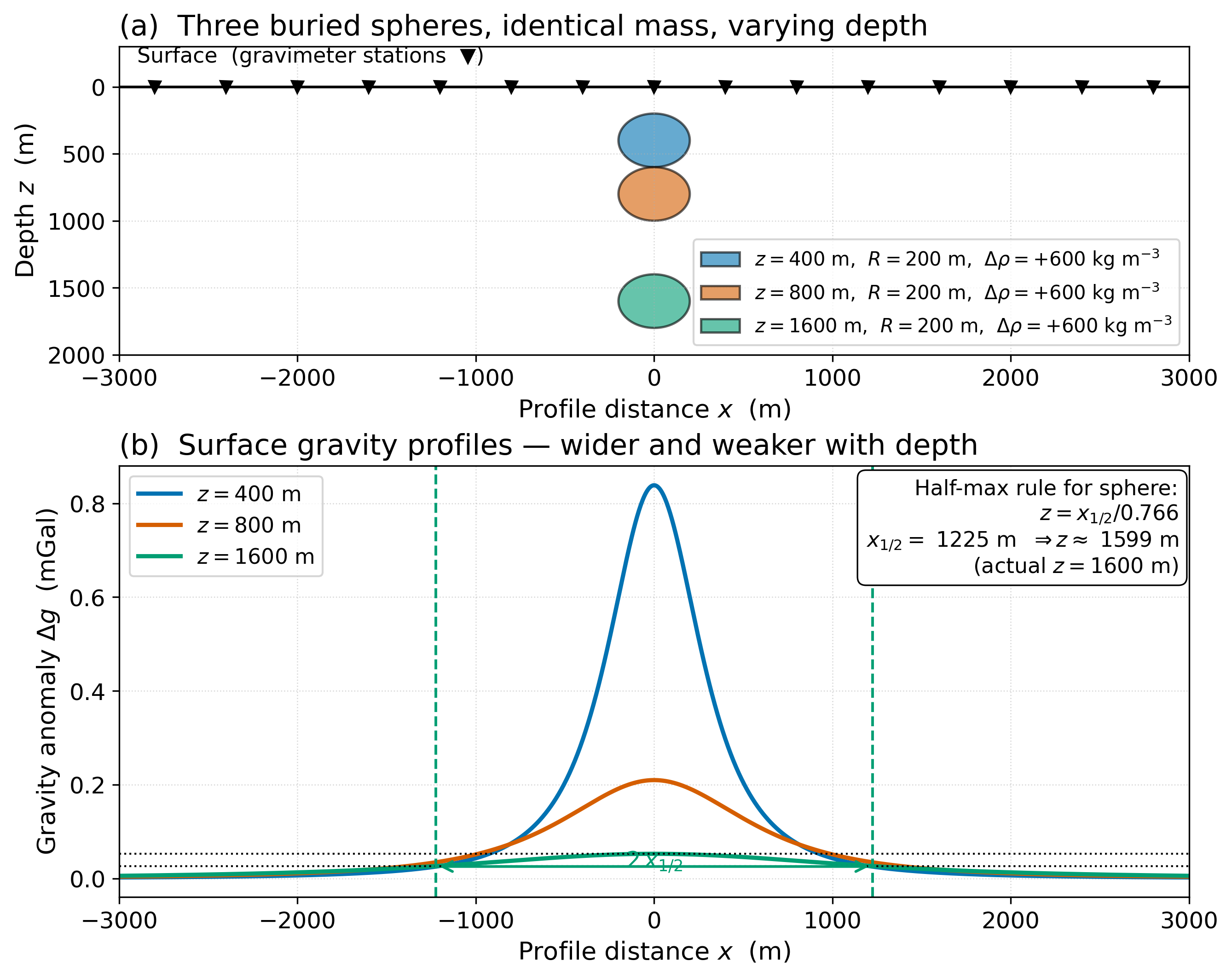— Fig. 91 The sphere anomaly is the canonical lesson in gravity interpretation. Three identical spheres at increasing depth produce signals that are *wider and weaker* — the depth-amplitude tradeoff. The half-maximum rule converts the measured width directly into a depth estimate, recovering the correct answer to better than 0.1% on the deep curve.#

3.2 Horizontal cylinder, finite slab, fault offset#

The closed-form expressions for the next three canonical shapes follow the same logic.

Horizontal cylinder (axis perpendicular to profile, e.g. a tunnel or a buried pipe, depth-to-centre \(z\)):

(159)#\[\Delta g(x) = \frac{2 G \lambda \, z}{x^{2} + z^{2}}, \qquad \lambda = \pi R^{2} \, \Delta\rho.\]

The amplitude falls off as \(1/(x^{2}+z^{2})\) rather than \(1/(x^{2}+z^{2})^{3/2}\) — slower decay, broader signature for the same depth. The half-max rule for a horizontal cylinder is \(x_{1/2} = z\) exactly.

Finite Bouguer slab (a horizontal layer of thickness \(\Delta z\) that exists only between \(x = x_{0}\) and \(x = x_{1}\)): a smooth positive bump centred on the slab, asymptoting to the infinite-slab limit \(2\pi G \Delta\rho \, \Delta z\) over the central region for slabs much wider than they are deep.

Vertical fault offset (a horizontal layer of contrast \(\Delta\rho\) vertically displaced by an amount \(\Delta z_{\text{throw}}\) across a fault at \(x = 0\)): an antisymmetric “step” in \(\Delta g\), with a positive lobe over the up-thrown side, a negative lobe over the down-thrown side, and a steepest gradient at the fault location itself.

These four shapes — and a handful of close relatives such as the dipping sheet — span most of the qualitative interpretations made in practice. Fig. 92 summarises their signatures.

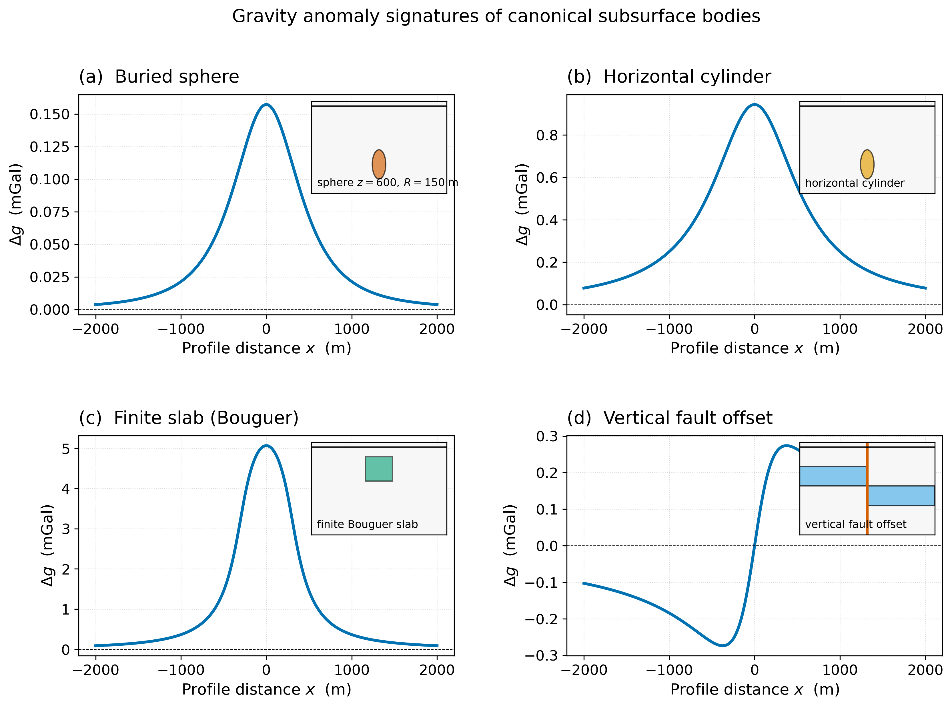
Fig. 92 The four canonical signatures of gravity interpretation. Each panel includes a small inset of the source geometry. Note that amplitude scales differ markedly: the slab anomaly is an order of magnitude larger than the sphere or cylinder, because superposition adds many small mass elements coherently.#

3.3 Regional and residual anomalies#

A real survey is typically dominated by a long-wavelength trend across the survey area — the regional anomaly — produced by deep-seated mass variations that interest tectonics but not the local geology. The wavelength of a gravity anomaly scales roughly with the depth to its source: a near-surface body produces a sharp, short-wavelength feature; a deep body produces a broad, gentle one.

The standard practice is to fit a low-order polynomial or a smooth surface to the regional trend, subtract it, and call what remains the residual anomaly. The residual is the input to subsurface-modelling efforts of the kind that recover salt-dome geometries, basin depths, or fault locations.

The choice of regional surface is a modelling choice, not a measurement; this introduces a degree of subjectivity that careful workers report transparently. A residual that depends sensitively on the choice of regional polynomial is, by that measure, less robust than one that does not.

3.4 The horizontal gradient — a tool for finding edges#

The horizontal derivative \(\partial \Delta g / \partial x\) peaks at the location of a vertical density contrast. Over a vertical fault, the gradient is largest directly above the fault plane; over a basin edge, the gradient peaks at the wall. The gradient is robust against long-wavelength trends, because differentiation suppresses the very-low-frequency components of the field. Map-view gradient images — easily produced from gridded gravity data — are widely used to locate structural lineaments that may not be obvious in the underlying anomaly map.

3.5 Comparing shapes at a common depth#

Before discussing measurement errors it is worth seeing the three localised signatures side by side at the same depth. Fig. 93 overlays a sphere, a horizontal cylinder, and a finite slab, all anchored to a depth-to-centre of \(z = 600\) m. The differences are subtle: at the half-maximum level the curves separate by less than a hundred metres, and they agree to within a few percent over the central region of the profile.

Two-panel figure comparing canonical gravity anomalies at a common depth. The left panel shows three normalised profiles (sphere in blue, horizontal cylinder in orange, finite slab in green), all peaking at one. Vertical dotted lines mark the half-width: about 460 m for the sphere (consistent with 0.766 z = 460 m) and about 600 m for the cylinder (consistent with x_half = z exactly). The slab falls between them and is flat-topped near x = 0. The right panel shows the same three profiles in absolute units in mGal: the cylinder peaks near 1.4 mGal, the slab near 0.75 mGal, and the sphere near 0.27 mGal. A grey band marks the typical land-survey measurement noise envelope of plus or minus 2 sigma (sigma = 0.05 mGal). The sphere anomaly drops into the noise band beyond about 600 m offset, while the cylinder and slab anomalies stay clearly above the noise out to roughly 1.6–2.1 km. 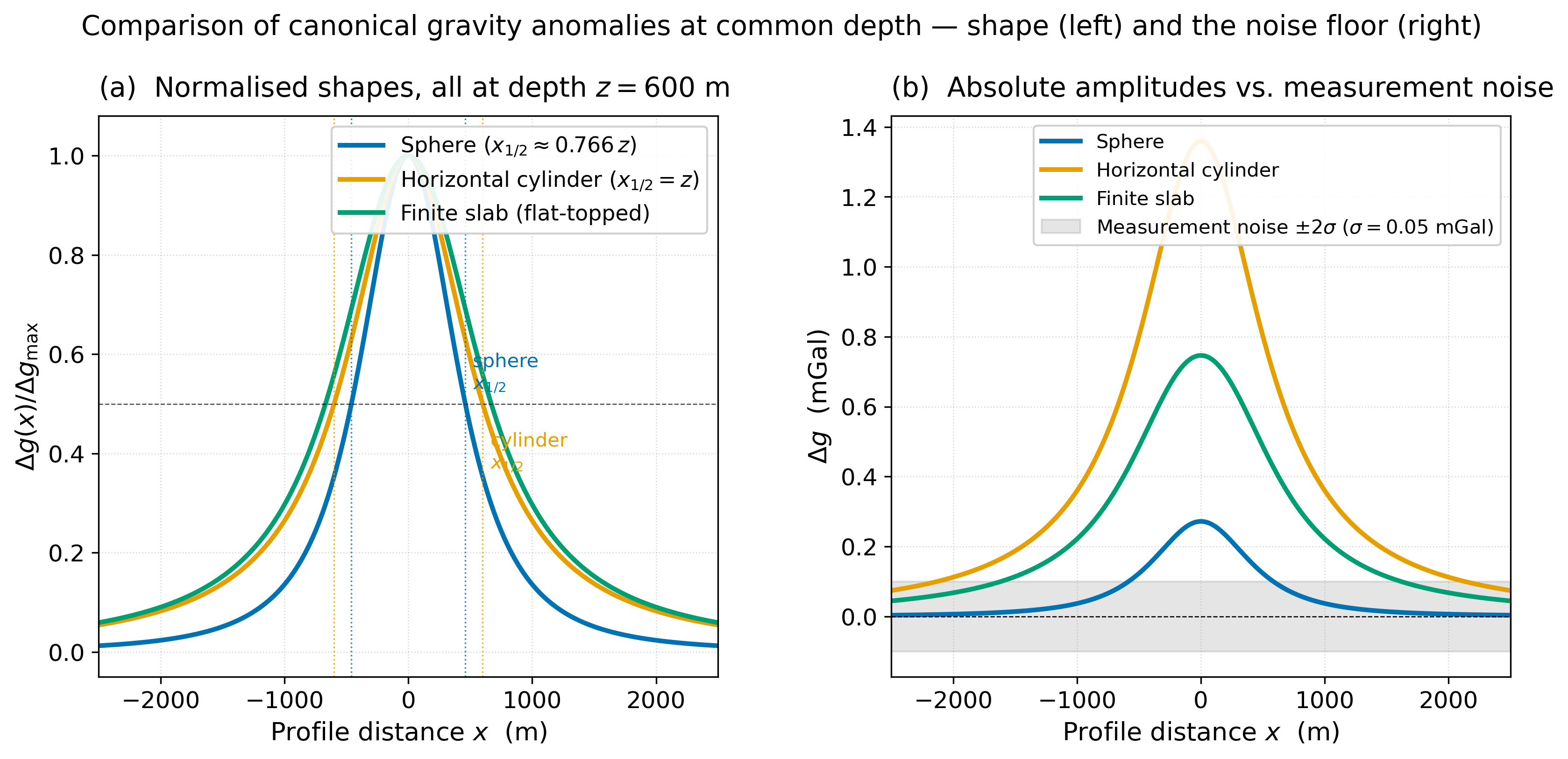— Fig. 93 The three localised anomaly shapes at \(z = 600\) m. **(a)** Normalised profiles isolate *shape*: the sphere falls off as \(1/r^{3}\) (steepest), the cylinder as \(1/r^{2}\) (broadest), and the finite slab is flat-topped near the centre. **(b)** Absolute amplitudes plotted together with a typical land-survey noise band (\(\sigma = 0.05\) mGal). At this depth, the sphere disappears into the noise beyond \(|x| \approx 600\) m, whereas the cylinder and slab remain detectable to several times that distance — a *survey-design* consequence of the slower far-field decay.#

The figure makes a point that is easy to miss when each shape is plotted in its own panel: for the same depth and density contrast, the amplitude spread between geometries is more than a factor of five, but the normalised shape difference is small. The choice of which closed-form to fit therefore matters more for amplitude-derived quantities (mass, density contrast) than for the half-max-derived depth.

3.6 Measurement errors and what they do to the inferred depth#

Field gravimeters are precise instruments — a modern relative LaCoste–Romberg or scintrex CG-6 reaches a repeatability of \(\sim 0.005\) mGal in the laboratory — but a real station gravity value carries error contributions from several sources that combine to a typical survey noise floor of \(\sigma_{\Delta g} \approx 0.05\) mGal, occasionally larger:

Instrument drift and tides. Mechanical drift of a few hundredths of a mGal per hour, plus solid-Earth tides of order ±0.3 mGal that must be removed by repeat base-station measurements and a tidal-correction model.
Station elevation and position. The free-air gradient is \(-0.3086\) mGal m⁻¹; a 30-cm error in station height costs about 0.1 mGal. A 1-metre horizontal position error in the latitude correction costs roughly 0.01 mGal at mid-latitudes.
Terrain correction error. Inadequate terrain models — particularly in mountainous surveys — leave residual amplitudes of 0.05–0.5 mGal.
Bouguer-density choice. The Bouguer slab correction is \(0.0419 \, \rho \, h\) mGal (with \(\rho\) in g cm⁻³ and \(h\) in m). Using \(\rho = 2.67\) versus \(\rho = 2.50\) g cm⁻³ on a 200 m elevation difference shifts the reduced anomaly by \(\sim 1.4\) mGal.

When these contributions are summed in quadrature, a well-run regional land survey delivers \(\sigma_{\Delta g}\) in the 0.05–0.10 mGal range. Modern absolute-gravity meters used for time-lapse work (FG-5, A10) push the floor below 0.005 mGal at a single station, at the cost of throughput.

The right panel of Fig. 93 shows what this means at depth. The sphere anomaly, the most rapidly decaying of the three signatures, drops into the \(\pm 2\sigma\) noise band beyond \(|x| \approx 600\) m at \(z = 600\) m — so for any source deeper than its own half-width, the tails of the anomaly are unrecoverable from a single profile.

Error propagation into the half-max depth. Suppose the peak amplitude is measured to \(\pm \sigma_{\Delta g}\). The half-maximum level \(g_{\max}/2\) is then known to \(\pm \sigma_{\Delta g}/2\), and the corresponding error in the half-width \(x_{1/2}\) is set by the local slope of the profile at the half-maximum point:

(160)#\[\sigma_{x_{1/2}} \;\approx\; \frac{\sigma_{\Delta g}/2}{|\partial \Delta g/\partial x|_{x_{1/2}}}.\]

For a sphere, \(|\partial g/\partial x|\) at \(x_{1/2}\) is \(\approx 0.55 \, g_{\max}/z\). Substituting and using \(z = x_{1/2}/0.766\), the relative error in depth is approximately

(161)#\[\frac{\sigma_{z}}{z} \;\approx\; 1.2 \, \frac{\sigma_{\Delta g}}{g_{\max}}.\]

In words: a noise-to-signal ratio of 5% propagates to a depth uncertainty of about 6%. For our salt-dome example in §6, \(g_{\max} = 16\) mGal and \(\sigma_{\Delta g} \approx 0.1\) mGal, giving \(\sigma_z / z \approx 0.7\%\) — well below the bias from the shape assumption. For a \(g_{\max} = 0.5\) mGal anomaly, however, \(\sigma_z/z\) climbs above 20%, and the half-max depth is dominated by measurement error rather than by the source geometry.

Key concept — when does noise dominate the depth?

The signal-to-noise ratio that matters for depth recovery is not the peak amplitude alone but \(g_{\max} / \sigma_{\Delta g}\) at the half-maximum. A rule of thumb:

\(g_{\max} / \sigma_{\Delta g} \gtrsim 50\): depth set by the geometry assumption; noise is a \(\lesssim 3\%\) contribution.
\(10 \lesssim g_{\max} / \sigma_{\Delta g} \lesssim 50\): depth uncertainty is \(\sim 5{-}15\%\); report the half-max depth with an explicit error bar.
\(g_{\max} / \sigma_{\Delta g} \lesssim 10\): the depth is essentially unconstrained by a single profile. Acquire more data, use the horizontal gradient (§3.4), or combine with seismic.

Deeper sources push the anomaly into this last regime even when the body is large: doubling \(z\) at fixed mass divides \(g_{\max}\) by four (sphere) or by two (cylinder), while \(\sigma_{\Delta g}\) is set by instrumentation and site conditions, not by the target.

3.7 From data error to model uncertainty — an ensemble of fits#

The half-max formula (§3.6) propagates noise into a single number, \(\sigma_z\). That is a useful first move, but it hides the shape of the uncertainty. The honest picture is that finite data error admits a family of models that fit the observations equally well — and the geometry of that family is the heart of how potential-field inverse problems are interpreted in practice.

Fig. 94 makes the family visible. A synthetic sphere anomaly is generated with the truth \((z^{*}, M^{*}) = (600\,\text{m}, 1.47\times 10^{10}\,\text{kg})\), then sampled at 31 stations spaced 100 m apart and contaminated with Gaussian noise of standard deviation \(\sigma_{\Delta g} = 0.05\) mGal. To assess which sphere parameters could have produced these data, every candidate \((z, M)\) pair on a coarse grid is scored by the reduced chi-squared,

(162)#\[\chi^{2}/N \;=\; \frac{1}{N}\sum_{i=1}^{N}\left(\frac{\Delta g_{i}^{\text{obs}} - \Delta g(x_{i}; z, M)}{\sigma_{\Delta g}}\right)^{2}.\]

A model is accepted if \(\chi^{2}/N \leq 1.5\) — heuristically, “fits the data within \(\sim 1.5\sigma\) on average.” This is a deliberately generous cutoff at this stage of the course; the geometry of the result, not its precise width, is what matters.

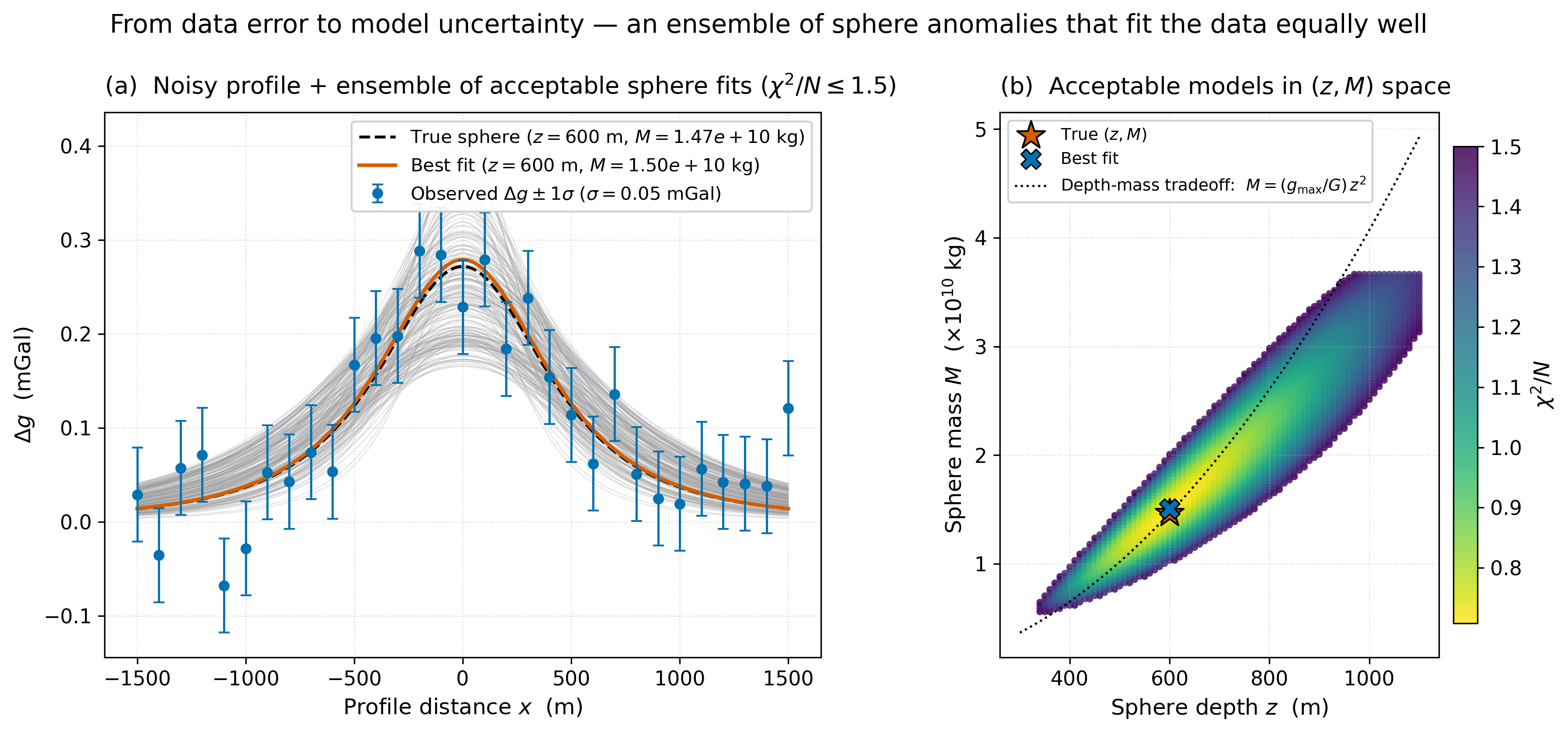
Fig. 94 From data error to model uncertainty. (a) Noisy observations (blue, with \(\pm 1\sigma\) bars). Every grey curve is a sphere model that satisfies \(\chi^{2}/N \leq 1.5\); the orange curve is the best fit. (b) The same accepted models plotted in \((z, M)\) space. The cloud is not a tight disc around the truth — it is a curved valley that follows the depth-mass tradeoff \(M = (g_{\max}/G)\,z^{2}\) (dotted line). Many of the models on this curve are nearly indistinguishable from the truth at the level of the data; gravity alone cannot tell them apart.#

Three lessons follow from Fig. 94.

The “answer” is a family, not a point. Any single best-fit estimate \((\hat z, \hat M)\) — the orange curve in the figure — is one member of the cloud, no more correct than the others. A scientific report should give either an explicit ensemble or, at minimum, the central value with marginalised uncertainties: \(\hat z = 600^{+220}_{-180}\) m, \(\hat M = (1.5 \pm 0.7) \times 10^{10}\) kg here.

Uncertainty in \(z\) and \(M\) is correlated, not independent. The cloud is a long ridge along the \(M \propto z^{2}\) direction — exactly the tradeoff predicted by the closed-form expression for \(g_{\max}\). Reporting \(\sigma_z\) and \(\sigma_M\) separately throws away most of the information; the joint uncertainty is the object of interest.

More data tightens the cloud — but only some of it. Adding stations far from the source narrows the cloud along the tradeoff valley (the tails of \(\Delta g\) are more sensitive to the long-range fall-off, which differs slightly between members of the family). Adding stations at the centre, where the profiles overlap most tightly, helps less. This is the survey-design corollary of error propagation and motivates the use of wide, sparse profiles rather than dense ones for deep targets.

This ensemble picture is the conceptual entry point to formal Bayesian inversion: a prior distribution on the model parameters, multiplied by the likelihood implied by the data and their errors, yields a posterior distribution whose shape is essentially the cloud in Fig. 94(b). For the geometric models of this lecture, the cloud can be sampled by brute-force grid evaluation as we have done; in higher-dimensional or non-linear problems (such as full-waveform inversion in Lecture 12 or geodynamic inversion in Lecture 25), the same logic is implemented with Markov-chain Monte Carlo or with ensemble Kalman methods. The accompanying notebook gravity_ensemble.ipynb lets students vary \(\sigma_{\Delta g}\), the survey aperture, and the depth and see the cloud expand, contract, and rotate accordingly.

Key concept — error propagation is correlated

In a parameter-fitting problem, finite data error never produces a tight disc around the truth. It produces a ridge aligned with the inherent tradeoffs of the forward map — here, \(M \propto z^{2}\). Reporting the answer as \(\hat z \pm \sigma_z\) and \(\hat M \pm \sigma_M\) independently overstates the uncertainty on each parameter and hides the correlation. The faithful representation is the ensemble itself, or its covariance matrix.

Key equation — what the gravity profile tells you

For interpretation, three numbers carry most of the information in a profile:

The peak amplitude \(g_{\max}\), which constrains the product \(\Delta\rho \cdot R^{3}\) for a sphere or \(\Delta\rho \cdot R^{2}\) for a cylinder.
The half-width \(x_{1/2}\), which constrains the depth \(z\).
The horizontal gradient \(\partial g/\partial x\), which locates edges — faults, basement contacts, intrusion margins.

4. The Forward Problem#

The forward problem in gravity is easy: given a parameterised subsurface model (a polygon and a density contrast, a sphere with prescribed centre and radius, or a stack of finite slabs), evaluate the integral of equation (156). For 2-D problems, the Talwani algorithm (1959) replaces an arbitrary polygon by a sum of triangular contributions whose closed-form gravity expressions are tabulated in any geophysics textbook. For 3-D problems with arbitrary shape, finite-element discretisation produces the same kind of forward map at the cost of a larger linear-algebra problem.

Two practical points anchor a forward-modelling workflow:

Density contrast, not density. The forward calculation is done with \(\Delta\rho\) relative to a background. If the background changes, every model parameter must be re-interpreted.
The forward map is linear in \(\Delta\rho\) and non-linear in geometry. Doubling \(\Delta\rho\) doubles the anomaly; doubling the depth changes the anomaly’s shape, not just its amplitude.

The companion notebook gravity_forward.ipynb implements equations (157) and (159) and a 2-D polygon (Talwani) forward modeller, and lets students vary the parameters interactively to develop intuition for how each parameter affects the predicted profile.

5. The Inverse Problem#

The inverse problem in gravity has three layers, each with its own kind of difficulty.

5.1 The geometric inverse — depth from width#

For a known shape (sphere, cylinder, dyke), the half-max rule and its relatives convert the measured width into a depth estimate. This is a one-line inverse problem in the sense that one number (the width) constrains one parameter (the depth). Errors in \(x_{1/2}\) translate directly into errors in \(z\), which makes the half-max approach robust at the qualitative level but prone to bias when the source is not actually the assumed shape.

5.2 The non-uniqueness theorem#

The deeper problem is that gravity is an integral observable. By Green’s third identity, two density distributions that differ by any harmonic function with vanishing exterior gradient produce identical surface gravity. Concretely, a thin shell at depth and a thicker, less dense layer at greater depth can be made to produce identical surface signals.

Three corollaries follow.

The total anomalous mass \(\int \Delta\rho \, dV\) is the only quantity uniquely determined by the surface field — and even this requires the survey to extend far enough beyond the body to capture the full anomaly (an integral constraint).
Increasing the depth of a body must be compensated by increasing its density contrast and/or its size. Without an independent constraint on one of these, the others cannot be separated.
The shape of an anomaly carries more information than its amplitude. A deep, dense source and a shallow, thin one produce the same peak amplitude but very different widths.

5.3 Residual interpretation in practice#

The Seattle Basin provides a near-canonical PNW example. The basin is filled with several kilometres of low-density Quaternary and Eocene sediments, producing a large negative isostatic-residual gravity anomaly. The width of the anomaly constrains basin depth; the asymmetry of the anomaly across the Seattle Fault Zone constrains the geometry of fault-related basin offset. Combining the gravity result with industry seismic profiles tightens the model substantially. The schematic in Fig. 95 shows the structure of the interpretation; the underlying open-access data are USGS public-domain.

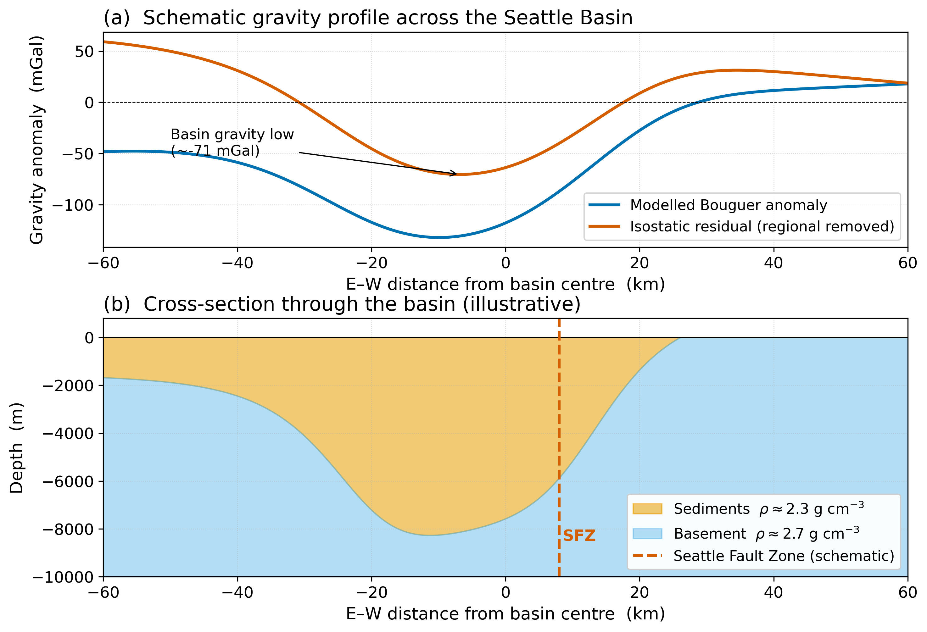
Fig. 95 Schematic isostatic-residual gravity anomaly across the Seattle Basin. The 60-mGal-amplitude residual is among the largest in western Washington and is the signal that first revealed the basin’s depth and asymmetry. The synthetic profile here illustrates the geometry; for the actual published data, see Brocher et al. (2017) and the open-access USGS gravity grid linked in §8.#

6. Worked Example — The Salt Dome at the Centre of the Practice Problem#

A coastal salt dome produces a near-circular Bouguer anomaly of \(g_{\max} \approx -16\) mGal with a half-width \(x_{1/2} \approx 3700\) m. Estimate the depth, radius, and approximate top of the salt body, given \(\rho_{\text{salt}} \approx 2.20\) g cm⁻³ and \(\rho_{\text{shale}} \approx 2.40\) g cm⁻³.

The negative anomaly tells us the body is less dense than its surroundings — consistent with a salt body in shale country. The density contrast is \(\Delta\rho = -200\) kg m⁻³.

From the half-max rule for a sphere,

\[ z = \frac{x_{1/2}}{0.766} = \frac{3700\,\text{m}}{0.766} \approx 4830\,\text{m}. \]

From the peak amplitude,

\[ g_{\max} = \frac{G M}{z^{2}} \;\Rightarrow\; M = \frac{|g_{\max}| \, z^{2}}{G} = \frac{16 \times 10^{-5} \cdot (4830)^{2}}{6.674 \times 10^{-11}} \approx 5.6 \times 10^{13}\,\text{kg}. \]

Setting \(M = \tfrac{4}{3}\pi R^{3} |\Delta\rho|\) and solving for \(R\):

\[ R = \left( \frac{3 M}{4 \pi |\Delta\rho|} \right)^{1/3} \approx 3800\,\text{m}. \]

The depth to the top of the salt body, treating it as a sphere of radius \(R\) centred at depth \(z\), is then \(z - R \approx 1000\,\text{m}\).

This is, of course, only a first-order interpretation. A salt dome is rarely spherical, the density contrast varies with depth, and the regional anomaly may have been imperfectly removed. A seismic line over the same body almost always tightens the depth-to-top estimate by a factor of two or more. But the gravity estimate is fast, cheap, and gets the order of magnitude right.

Concept check

Two anomalies have identical peak amplitude (\(g_{\max} = +5\) mGal) but different half-widths: \(x_{1/2,\text{A}} = 200\) m and \(x_{1/2,\text{B}} = 2000\) m. Estimate the depth of each source assuming both are spheres. What is the implied difference in source mass?
A profile across a vertical fault shows an antisymmetric gravity step of total amplitude \(\Delta g = 4\) mGal. The horizontal gradient \(|\partial g/\partial x|_{\max}\) peaks at the inferred fault location at \(0.5\) mGal per kilometre. What does this gradient tell you that the step amplitude does not?
You apply two different regional polynomials (1st and 2nd order) to the same dataset and compare the residual anomalies over an inferred salt dome. The half-width changes by 30 % and the peak amplitude by 15 %. What does this tell you about the reliability of the depth and density estimates derived from the residual?

7. Course Connections#

Backward to Lecture 19, whose Bouguer reduction provides the input \(\Delta g_{CB}\) that this lecture interprets.
Backward to Lectures 10–12 (Migration, Whole Earth Imaging, Seismic Tomography), which establish the vocabulary of forward and inverse problems. The non-uniqueness theme of this lecture parallels the resolution-vs-uniqueness tradeoff in tomography.
Forward to Lecture 21, where the long-wavelength part of the Bouguer field is reinterpreted as evidence for isostatic compensation.
Forward to Lecture 23 (Earth’s Magnetism), where the same forward-and-inverse logic is applied to magnetic anomalies, and joint gravity-magnetic modelling becomes the standard interpretation tool in basement studies.
Lab connection to Lab 5 (Gravity Surveys), which uses Python implementations of the forward maps in this lecture to reproduce a published anomaly profile.

8. Research Horizon#

Three open-access threads bring this lecture into contact with current research.

Open-access gravity data for the Pacific Northwest. The USGS gravity data portal (https://mrdata.usgs.gov/services/gravity) provides the full national point-data archive in public domain. Brocher et al. (2017) integrated these data with seismic and geodetic constraints to produce a regional model of crustal blocks and their rotation; the paper is open access through AGU at https://doi.org/10.1002/2016TC004223.

Deep-learning-assisted gravity interpretation. A 2023 review by Linsel et al. in Geophysics (open-access preprint at https://arxiv.org/abs/2306.04036) discusses convolutional neural networks for fault-edge detection in gridded gravity and magnetic data, framing the approach as a high-throughput first pass that reduces — but does not eliminate — the need for human interpretation.

Joint gravity–geodynamics inversion. Steinberger et al. (2022, Earth and Planetary Science Letters 591, 117602; open access at https://doi.org/10.1016/j.epsl.2022.117602 (⚠ DOI returns 404 — verify manually)) use mantle-convection-derived density predictions as a forward operator for global gravity inversion, demonstrating that long-wavelength gravity contains information about flow, not only density. The result is a useful corrective to the often-implicit assumption that a measured anomaly maps to a static density distribution.

9. Societal Relevance — The Seattle Basin and Earthquake Hazard#

The Seattle Basin’s gravity signature — a \(\sim 60\)-mGal residual low — is more than a curiosity. The same low-density sediments that produce the gravity anomaly amplify the long-period ground motion produced by Cascadia subduction-zone earthquakes by factors of 3–5 relative to a hard-rock site. The basin’s geometry, recovered partly from gravity, is now the input to ground-motion simulation codes used in the regional probabilistic seismic hazard analysis (PSHA) for greater Seattle.

USGS Open-File Report 2018-1149 (Frankel et al., 2018, public domain; https://pubs.usgs.gov/of/2018/1149/) summarises the basin-amplification problem and its propagation through PSHA into building-code design ground motions. The shape of the basin matters: a deeper, more asymmetric basin amplifies surface waves differently than a shallower, more symmetric one. Improvements in gravity interpretation feed directly into seismic-hazard estimates, which feed directly into building-code provisions for the Puget Sound region.

AI Literacy — AI Epistemics#

A useful exercise that will appear in the lab and the discussion section asks students to query a general-purpose LLM with the prompt: “Derive the gravity anomaly above a buried sphere. Give the half-width-to-depth relation and explain why the anomaly is non-unique.”

The exercise is diagnostic. A good response derives the formula in equation (157), recovers \(x_{1/2} \approx 0.766\,z\), and articulates the depth-density tradeoff. A poor response produces formulas that look plausible but include subtle errors — a missing factor of \(z\), a wrong exponent on the denominator, a confusion between sphere and cylinder. These errors are not detectable from the formula’s appearance alone; they are detectable only by checking dimensional consistency, by comparing the predicted half-width-to-depth ratio against the textbook value, or by running the formula on a forward model with known parameters and verifying that the recovered depth matches the input.

This is the central principle of AI epistemics in physical science: trust by verification, not by appearance. An LLM trained on generic web text has no internal geometric understanding of the inverse-square law; it has statistical patterns that look like derivations. The patterns are usually correct, occasionally wrong in ways that compound through the analysis. A student who treats LLM output as a starting point for their own derivation — and who checks the result against an independently-known limiting case — gets the speed benefit of the tool without the silent-error risk.

A useful open-access entry point on the broader topic is the Geophysics Reproducibility Manifesto of the SCOPED community (https://scoped.codes), which establishes computational-reproducibility norms for the publication of inverse problem results.


Course LOs addressed	LO-1, LO-2, LO-3 (forward/inverse), LO-4, LO-5 (computational tools)
Learning outcomes practiced	LO-OUT-A, LO-OUT-B, LO-OUT-C, LO-OUT-D (set up an inverse problem), LO-OUT-E (interpret residuals)
Prior lecture	L19 — Earth’s Gravity Field and the Geoid
Next lecture	L21 — Isostasy and Lithospheric Flexure
Lab connection	Lab 5 — Gravity Surveys (GravMag-style polygonal modelling in Python)
Discussion	Session 5 — Gravity, Ice Sheets, and CO₂