Ground Motions, Intensities, and Building Damage

Ground Motions, Intensities, and Building Damage#

Prerequisites#

Students should be comfortable with: the magnitude scale and seismic moment from Lecture 15; the wave equation and the concepts of P-, S-, and surface-wave amplitude and frequency from Lectures 3–5; a base-ten logarithm; and the single-degree-of-freedom oscillator with natural period \(T_0 = 2\pi\sqrt{m/k}\) from introductory physics.

1. The framing question: how do we describe the shaking?#

The 28 February 2001 Nisqually earthquake released a moment magnitude \(M_W\) 6.8 from a focal depth of 52 km beneath the southern Puget Sound. The number \(M_W\) 6.8 captured the source: how much fault slipped, over what area, multiplied by crustal rigidity. But the people sheltering under desks in Olympia and Seattle did not experience \(M_W\) 6.8. They experienced ground motion — a particular acceleration history at their particular building, on their particular soil, lasting roughly 30 seconds and with a peak horizontal acceleration of about 0.16 g downtown and rather more in the Duwamish industrial flats.

That distinction is the centre of this lecture. A magnitude is one number assigned to the source. A ground motion is a function of time recorded at a station. An intensity is a description of the human experience or the engineering damage at a location. None of these is reducible to the others, and confusion among them is the most common single error in popular accounts of earthquakes.

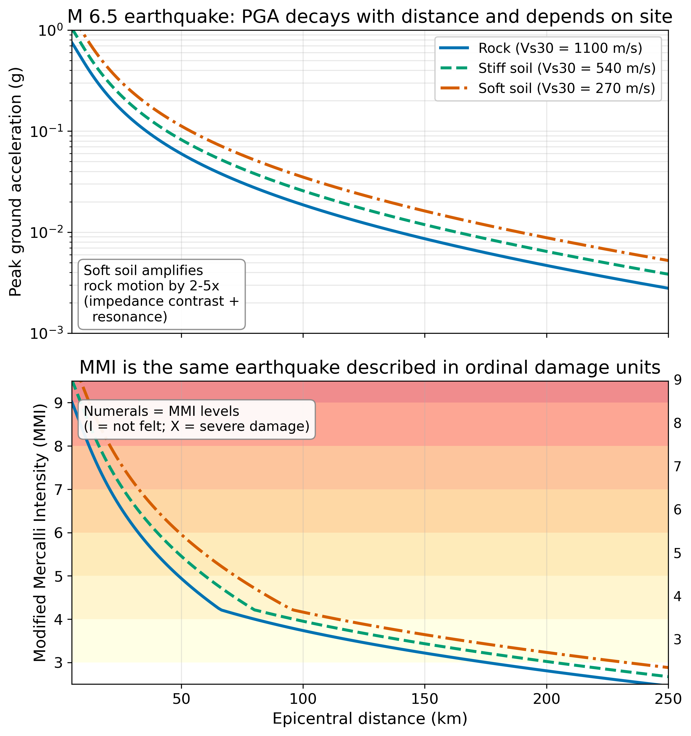
Two stacked plots. Top: peak ground acceleration on the vertical axis versus epicentral distance on the horizontal axis, with three labelled curves for soft soil, stiff soil, and rock; PGA decreases with distance and is highest on soft soil. Bottom: the same axes for Modified Mercalli Intensity, decreasing in steps from IX near the source to II at 200 km, with shaded bands. — Fig. 80 Two complementary descriptions of shaking. **Top:** peak ground acceleration, an instrumental measurement, decays roughly as a power of distance and depends strongly on near-surface site conditions. **Bottom:** Modified Mercalli Intensity, an ordinal description of felt shaking and damage, also decays with distance but in discrete integer steps that aggregate over a wide range of physical amplitudes. The two scales are linked statistically through Ground Motion / Intensity Conversion Equations (GMICEs) of the form used in USGS ShakeMap. Reproduces the qualitative content of slide 4 of the legacy deck and slide 6 (PGA/PGV/PGD/\(S_a\) definitions); mathematical curves are computed from a synthetic attenuation model parameterised after Worden et al. (2012).#

The lecture proceeds in three movements. Sections 2–3 define the physical observables — PGA, PGV, PGD, and spectral acceleration — and the framework that connects them through Newton’s second law to the forces on a building. Sections 4–5 turn from instruments to felt experience: the Modified Mercalli scale, isoseismal maps, and the limits of intensity as a measure of “size.” Sections 6–7 explain why the same earthquake shakes adjacent buildings differently — site amplification, resonance, liquefaction — and how engineers convert that knowledge into the seismic provisions of modern building codes.

2. Governing physics: from the wave equation to a force on a building#

A seismic wave reaches a station as a vector ground motion \(\boldsymbol{u}(\boldsymbol{x}, t)\). Three derivatives of that single field generate every quantity in this lecture:

Key Concept — Three time derivatives, three quantities

For a ground-motion record measured at position \(\boldsymbol{x}\):

\[ \boldsymbol{u}(\boldsymbol{x}, t)\quad\xrightarrow{\partial/\partial t}\quad \boldsymbol{v}(\boldsymbol{x}, t) = \dfrac{\partial \boldsymbol{u}}{\partial t} \quad\xrightarrow{\partial/\partial t}\quad \boldsymbol{a}(\boldsymbol{x}, t) = \dfrac{\partial^2 \boldsymbol{u}}{\partial t^2}. \]

The three are linked by Fourier transformation: at angular frequency \(\omega\), \(\hat{v} = i\omega\,\hat{u}\) and \(\hat{a} = -\omega^2\,\hat{u}\). A factor of \(\omega\) in the spectrum amplifies the high-frequency content at each step. Therefore:

Displacement \(u\) emphasises long periods (large eddies of the wavefield, surface waves at distance, static offset of permanent deformation).
Velocity \(v\) emphasises intermediate periods (the body of the shaking, roughly 0.3–3 s for crustal earthquakes).
Acceleration \(a\) emphasises short periods (sharp arrivals, high-frequency body waves). By Newton’s second law, \(\boldsymbol{F} = m\boldsymbol{a}\), the acceleration is also the force-per-unit-mass that the ground exerts on a rigid object resting on it.

The three peak amplitudes of these signals are called peak ground acceleration (PGA), peak ground velocity (PGV), and peak ground displacement (PGD). Strong-motion engineering uses the maximum horizontal value of each, taken either as the larger of the two recorded horizontal components or, in modern practice, as the maximum over all azimuths obtained by rotating the two horizontal traces through 360° (the “RotD100” measure of @Boore2010).

A real building, however, does not respond uniformly to all frequencies. A flagpole, a single-storey house, and a 60-storey tower each have a characteristic natural period of vibration — the period at which they sway most easily in response to any forcing. The quantity that most directly governs how much that flagpole or that tower will be excited is not PGA itself but 5%-damped pseudo-spectral acceleration \(S_a(T)\): the peak acceleration a single-degree-of-freedom oscillator of natural period \(T\) would experience while sitting on this ground. Mathematically, \(S_a(T)\) is the maximum of the response of the equation

(128)#\[ \ddot{x}(t) + 2\zeta\omega_0\,\dot{x}(t) + \omega_0^2\,x(t) \;=\; -\,\ddot{u}_g(t), \qquad \omega_0 = 2\pi/T, \]

where \(x(t)\) is the deflection of the oscillator’s mass relative to its base, \(\ddot{u}_g(t)\) is the recorded ground acceleration, \(\zeta = 0.05\) is the standard damping ratio used in design codes, and \(S_a(T) \equiv \omega_0^2\,\max_t |x(t)|\) has units of acceleration (commonly reported in \(g\)). Building codes specify design values of \(S_a(T)\) at \(T = 0.2\) s (short-period, governing low-rise structures) and \(T = 1.0\) s (long-period, governing taller buildings), often with values at \(T = 3.0\) s as well for very tall structures.

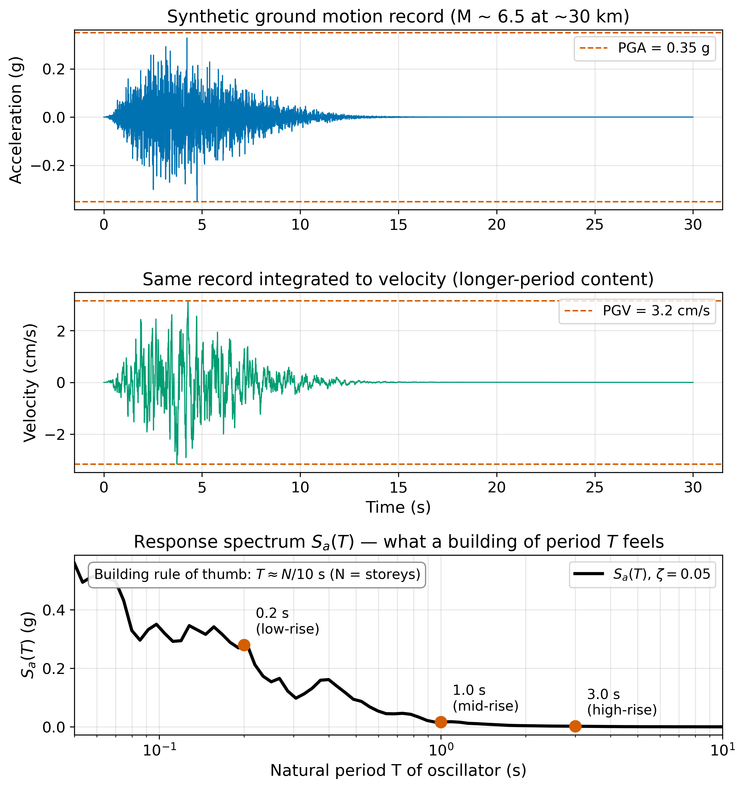
Three panels stacked vertically. Top: a synthetic ground acceleration time series, lasting about 30 seconds, with a maximum near 5 seconds. Middle: the same record as ground velocity, with longer-period oscillations. Bottom: the 5%-damped pseudo-spectral acceleration as a function of period from 0.05 to 10 seconds, showing a broad peak between 0.2 and 1 second. — Fig. 81 The journey from a recorded ground motion to a design quantity. The top panel shows a synthetic acceleration record. Integrating once in time gives the velocity (middle), whose longer-period content is visible. The bottom panel shows the 5%-damped response spectrum \(S_a(T)\) — the peak acceleration that an idealised single-degree-of freedom oscillator of natural period \(T\) would experience under this shaking. A building of period \(T\) feels the shaking most strongly at the height of its corresponding peak; a stiff one-storey house (\(T \approx 0.1\) s) and a 60-storey tower (\(T \approx 7\) s) read quite different “intensities” of the same earthquake.#

2.1 The rule of thumb: \(T_{\text{building}} \approx N/10\) s#

Decades of measurements on real buildings — most systematically compiled by ATC-72 and quoted in @Lowrie2020 — show that the fundamental period of a regular framed building scales approximately linearly with its number of storeys \(N\):

(129)#\[ T_{\text{building}} \approx \frac{N}{10}\,\text{s}. \]

A two-storey wood-frame house has \(T \approx 0.2\) s and is excited strongly by PGA-rich high-frequency shaking. The 60-storey Columbia Tower in Seattle has \(T \approx 6\) s and barely feels a typical crustal \(M_W\) 6 earthquake, but is excited efficiently by the long-period surface waves of a Cascadia \(M_W\) 9 — for which it must be designed. The Tokyo Skytree at 634 m has \(T \approx 10\) s; the Akashi-Kaikyō suspension bridge has \(T = 8\)–\(20\) s. As cities have built taller, their resonant periods have lengthened and the relevant ground-motion band has shifted to longer periods — precisely the band where megathrust subduction earthquakes radiate most efficiently.

3. Mathematical framework: site amplification#

Why should the same wave shake adjacent buildings differently? Two adjacent stations on rock and on soft soil can record peak velocities that differ by a factor of two to five. The physics is captured by the impedance contrast between the deep crustal rock through which the wave travels and the shallow sediments through which it must emerge.

3.1 Energy flux and the impedance ratio#

Consider an SH wave propagating vertically upward through a half-space of seismic impedance \(Z_1 = \rho_1 \beta_1\) (density times shear-wave velocity) and refracting into a shallow soft layer of impedance \(Z_2 = \rho_2 \beta_2\), with \(Z_2 \ll Z_1\). The transmitted-wave amplitude \(A_2\) at the surface — accounting for the free-surface reflection that doubles it — relates to the incident amplitude \(A_1\) in the rock by

(130)#\[ \frac{A_2}{A_1} \;=\; \frac{2\,Z_1}{Z_1 + Z_2} \;\approx\; \frac{2\,Z_1}{Z_1}\;=\;2, \qquad\text{(if }Z_2\ll Z_1\text{)}, \]

a factor of two amplification before any resonance is considered. For a 30-m-thick layer of soft mud over crystalline basement (\(\beta_2 \approx 200\) m/s, \(\rho_2 \approx 1700\) kg/m³ versus \(\beta_1 \approx 3500\) m/s, \(\rho_1 \approx 2700\) kg/m³), the impedance ratio is \(Z_1/Z_2 \approx 28\) and equation (130) predicts an amplification of \(\sim 2\) for the upgoing wave. This is the single-layer linear prediction; real soft soils amplify more at their resonant frequencies and less at other frequencies, and they deamplify when the shaking exceeds their elastic limit.

3.2 Site resonance#

A flat-lying soft layer of thickness \(H\) over rigid rock acts as a quarter-wavelength resonator for vertically propagating SH waves. The fundamental resonance condition is

(131)#\[ H \;=\; \frac{\lambda}{4} \;=\; \frac{\beta_2}{4\,f_0}, \qquad f_0 \;=\; \frac{\beta_2}{4\,H}. \]

The Duwamish industrial flats in Seattle, for instance, sit on \(H \approx 200\) m of unconsolidated sediment with average \(\beta_2 \approx 350\) m/s, predicting \(f_0 \approx 0.4\) Hz — a period of \(T_0 \approx 2.3\) s, dangerously close to the natural period of 20–30-storey buildings. The 1985 Mexico City earthquake, in which the deep lacustrine clay basin amplified \(T \approx 2\)-s motion by factors approaching 50 and selectively destroyed mid-rise buildings, is the canonical illustration.

Notation

Symbol	Meaning	Units
\(u, v, a\)	ground displacement, velocity, acceleration	m, m/s, m/s²
PGA, PGV, PGD	peak ground acceleration, velocity, displacement	\(g\) or m/s², cm/s, cm
\(S_a(T)\)	5%-damped pseudo-spectral acceleration at period \(T\)	\(g\) or m/s²
\(T\)	period (of an oscillator or of a wave)	s
\(\omega = 2\pi/T\)	angular frequency	rad/s
\(\zeta\)	damping ratio (0.05 = 5%)	—
\(\rho\), \(\beta\)	density, shear-wave velocity	kg/m³, m/s
\(Z = \rho\beta\)	seismic impedance	kg m⁻²s⁻¹
\(H\)	thickness of soft layer	m
\(f_0 = \beta_2/(4H)\)	fundamental site resonance frequency	Hz
\(N\)	number of building storeys	—
\(V_{S30}\)	average \(S\)-wave speed in upper 30 m	m/s
\(I_{\text{MMI}}\)	Modified Mercalli Intensity	I–XII (ordinal)

4. The forward problem: ground-motion prediction#

Given an earthquake with magnitude \(M\), distance \(R\) from the station, and site parameter \(V_{S30}\) (the time-averaged shear-wave velocity in the upper 30 m), can we predict PGA, PGV, and \(S_a(T)\)? This is the forward problem of engineering seismology, and its empirical solution is the Ground-Motion Prediction Equation (GMPE), a regression of observed records on these source, path, and site variables. A schematic GMPE has the form

(132)#\[ \ln Y \;=\; f_{\text{source}}(M)\;+\;f_{\text{path}}(M, R)\;+\;f_{\text{site}}(V_{S30}) \;+\; \varepsilon, \]

where \(Y\) is the ground-motion intensity measure (PGA, \(S_a(T)\), etc.) and \(\varepsilon\) is a residual with standard deviation \(\sigma \approx 0.6\) in natural-log units — a factor of \(e^{0.6} \approx 1.8\) in linear amplitude. Even with the best modern GMPEs, predicted motions and observed motions disagree by a factor of two on a routine basis. That irreducible scatter is fundamental to the forecasting problem and propagates into every seismic-hazard map.

The USGS ShakeMap system @Worden2020 implements the forward problem in near-real time after every felt earthquake. It takes the rapidly estimated source, predicts ground motion everywhere using a chosen GMPE, and then conditions the prediction on whatever observed PGAs, PGVs, and felt-intensity reports are available — a Bayesian update of the prior GMPE prediction. ShakeMap is the operational embodiment of equations (132) and the impedance/resonance ideas of §3.

5. The inverse problem: from observation to source — the modern intensity scale#

For an earthquake recorded only by historical descriptions (newspapers, diaries, structural damage reports), no instrumental PGA exists. The only available observable is the human or engineering response: was there panic? Did chimneys fall? Did masonry collapse? The Modified Mercalli Intensity (MMI) scale, a revision by @Wood1931 of the original 12-point scale of Mercalli (1902), is the standard ordinal description of these effects (Table 1).

Table 2 Modified Mercalli Intensity scale (paraphrased from USGS public-domain definitions).#
Level	Effect	Approx. PGA
I	Not felt except by very few	\(< 0.0017\,g\)
III	Felt by people indoors, vibrations like a passing truck	\(\sim 0.005\,g\)
V	Felt by all; some dishes broken, plaster cracks	\(0.04\)–\(0.09\,g\)
VI	Felt by all; furniture moved, slight damage	\(0.09\)–\(0.18\,g\)
VII	Damage negligible in well-built structures, considerable in poorly built	\(0.18\)–\(0.34\,g\)
VIII	Damage slight in specially designed structures, great in poorly built	\(0.34\)–\(0.65\,g\)
IX	Damage considerable in specially designed structures	\(0.65\)–\(1.24\,g\)
X	Most masonry destroyed; rails bent	\(> 1.24\,g\)

Three properties of intensity follow from the table.

It is ordinal, not interval. The step from VI to VII is not the same physical jump as VII to VIII. Statistical relations between intensity and PGA must therefore be estimated, not assumed — @Worden2012 calibrated the modern Ground Motion / Intensity Conversion Equation (GMICE) from thousands of paired California records and DYFI reports, fitting a piecewise linear regression of MMI on \(\log_{10}\text{PGA}\) and on \(\log_{10}\text{PGV}\).

It mixes source, path, and site. A wood-frame house in Olympia on glacial outwash and an unreinforced-masonry building in Seattle on the Duwamish flats will report different MMI values for the same event. Felt-shaking maps (USGS Did You Feel It?) therefore reveal both the earthquake and the geology.

It depends on the building stock. The Mercalli scale was calibrated against early-twentieth-century unreinforced-masonry construction. Modern wood-frame houses fail at higher intensities than the original scale assumes; modern URMs collapse at lower values. The same shaking is reported as a different MMI in San Francisco today than it would have been in 1906.

These three caveats explain Robert Mallet’s old warning, repeated throughout the field: intensity is not a measure of an earthquake, it is a measure of an earthquake at a place.

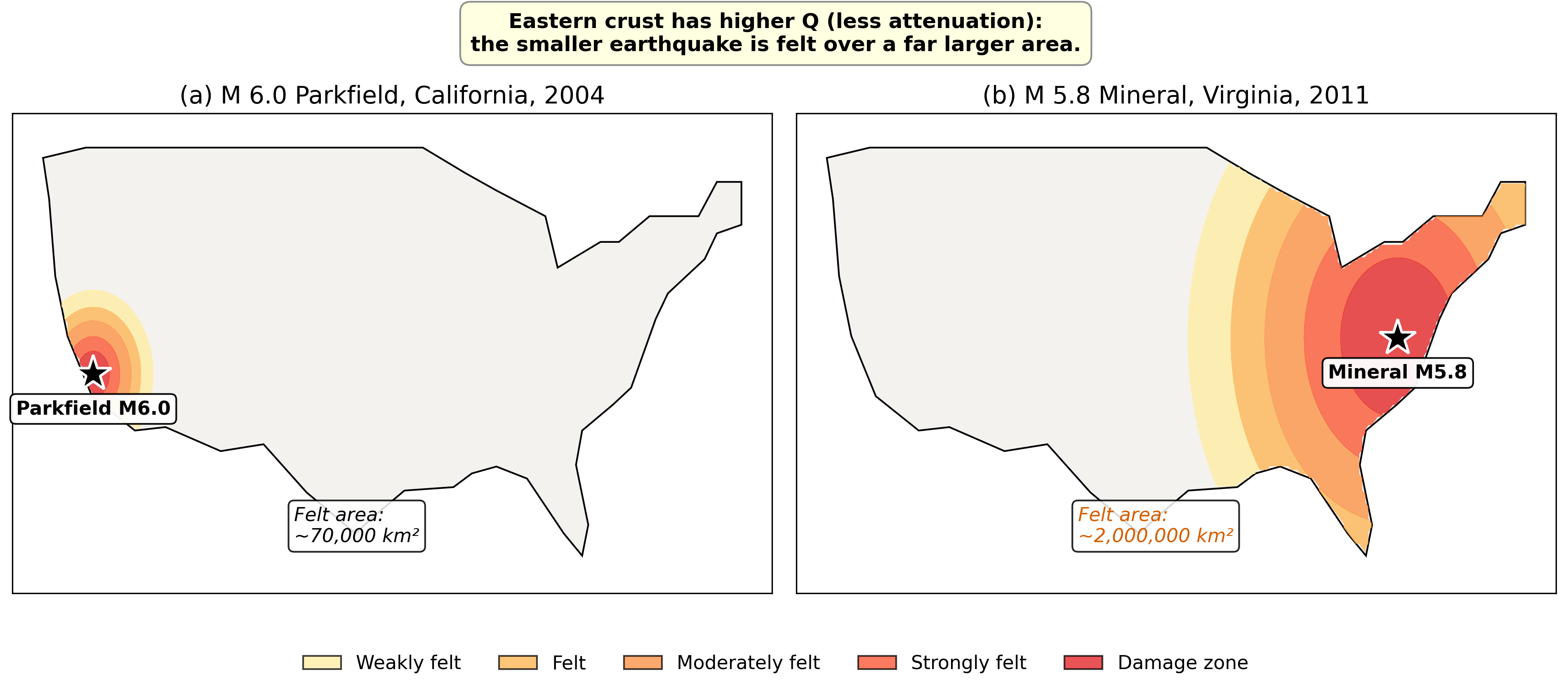
Two side-by-side outline maps of the contiguous United States. Left panel labelled "M6.0 Central California 2004" shows felt-it markers concentrated within roughly 200 km of the central California coast. Right panel labelled "M5.8 Central Virginia 2011" shows felt-it markers spread across the entire eastern half of the continent. — Fig. 82 Two earthquakes of similar magnitude, vastly different felt areas. The 2004 Parkfield, California, \(M_W\) 6.0 was felt across a region roughly 300 km in diameter. The 2011 Mineral, Virginia, \(M_W\) 5.8 was felt across more than 2 million km², from Atlanta to Toronto. The difference is not the source: it is the path. The eastern North-American crust has a quality factor \(Q\) several times larger than the western United States, and seismic waves attenuate far less per unit distance. Reproduces the qualitative content of slide 9 of the legacy deck using synthetic isoseismal contours parameterised after USGS *Did You Feel It?* data products.#

6. Site effects and soil failure#

6.1 Liquefaction#

In saturated, loosely packed sand, prolonged shaking causes the intergranular water pressure to rise faster than it can drain. When the pore pressure \(p\) approaches the effective confining stress \(\sigma' = \sigma - p\), the granular skeleton temporarily loses contact and the deposit flows like a liquid. This is liquefaction, and three conditions favour it:

Loose sandy soil below the water table.
Strong, sustained shaking (PGA \(\gtrsim 0.1\,g\) for at least 10 cycles).
Shallow ground water (within a few metres of the surface).

The 1964 Niigata earthquake, the 2011 Christchurch earthquake, and sections of the 1989 Loma Prieta and 2001 Nisqually events all produced spectacular liquefaction. The physical signature — sand boils at the surface, buildings settling or tilting on intact foundations — distinguishes liquefaction damage from direct shaking damage. In Seattle, the Duwamish flats and Harbor Island are mapped liquefaction-prone areas; the Washington Geological Survey’s Liquefaction Susceptibility of Washington maps are derived from exactly this physical reasoning combined with \(V_{S30}\) and depth- to-water-table compilations.

6.2 Building failure modes#

Damage in framed buildings has a small number of recurring patterns, each diagnostic of a particular mismatch between the input ground motion and the building’s resistance:

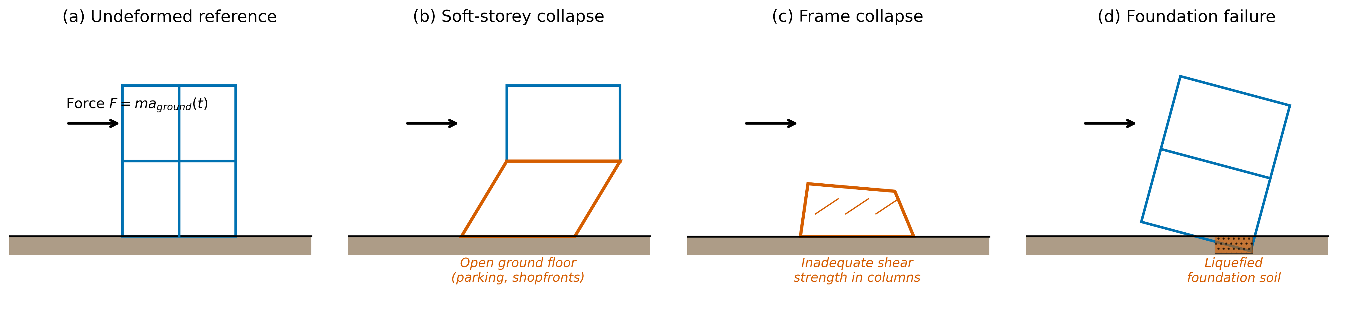
Four side-by-side line drawings of a two-storey building. From left to right: undeformed reference, soft-story collapse with ground floor sheared sideways, full collapse with roof on the ground, and foundation rotation with the building tilted as a rigid body. Each drawing is labelled and shows arrows for the input force. — Fig. 83 Four characteristic failure modes of framed buildings under strong shaking. **Soft-storey collapse** localises the deformation in a single weak floor — typically the ground floor of a building with parking openings — leading to total loss of that floor. **Frame collapse** results from inadequate shear strength in the lateral load path. **Foundation failure** can be uniform settlement, tipping, or differential — the latter being the most damaging because it introduces internal stresses absent in pure rigid-body motion. The geometry redrawn from the slide deck of the legacy course; the deformation kinematics computed from a Timoshenko-beam idealisation.#

The engineering counterpart to each failure mode is a retrofit strategy: shear walls (vertical reinforced concrete elements between window openings) defeat soft-storey collapse; cross-bracing or gussets add shear strength to existing frames; base isolation (laminated rubber-and-steel bearings beneath the foundation) decouples the building from the ground motion and shifts the building’s effective natural period upward, away from the high-frequency band where most shaking energy lives; viscous dampers convert kinetic energy into heat.

7. Connecting to Cascadia: ground motions in the Pacific Northwest#

The Pacific Northwest faces three distinct earthquake source populations, each generating a characteristic ground-motion signature. Crustal earthquakes on faults such as the Seattle Fault produce relatively short-duration, high-frequency shaking; their PGA can be large (the 2001 Nisqually deep-slab event reached \(\sim 0.3\,g\) at some Olympia stations) but \(S_a(T)\) at long periods remains modest. Intraslab earthquakes within the subducting Juan de Fuca plate, of which Nisqually is the canonical example, occur deep enough that high-frequency surface motion is attenuated by several orders of magnitude over the path. Megathrust earthquakes on the plate-interface — last in 1700, expected at unknown future date — radiate enormously long-period energy (\(T = 3\)–\(30\) s) over durations of two to five minutes. The same Cascadia \(M_W\) 9 will produce relatively modest PGA at Seattle but record-setting \(S_a(3\text{ s})\) — exactly the band that excites the city’s high-rise inventory.

The PNSN’s nearly 200 strong-motion stations across Washington and Oregon provide the ground-truth data that constrain the GMPEs used in the Washington Department of Natural Resources’ tsunami- and shaking-hazard maps. This is the inverse problem in operational form: instrument the network densely, accumulate a record set, regress the GMPE, and use it to forecast where an as-yet-unrecorded \(M_W\) 9 will most strongly damage the built environment.

8. Research Horizon#

Three open frontiers in strong-motion seismology drive much of the current literature. They are all areas where geophysics intersects machine learning, real-time computation, and engineering decision- making.

Site-specific GMPEs from machine learning. The largest residuals in equation (132) come from the assumption that a single parameter (\(V_{S30}\)) captures all site effects. Modern work uses full \(V_S\) profiles, deep-learning-based site classifications, and microtremor horizontal-to-vertical spectral ratios to fit station-specific corrections — typically halving the residual at well-instrumented sites @Bahrampouri2024.

Earthquake early warning. The USGS ShakeAlert system, deployed across Washington, Oregon, and California in 2021–2023, uses the first few seconds of P-wave arrivals at the closest stations to estimate magnitude and predict the ground motion that the S and surface waves will produce moments later. Machine-learning models trained on the entire global strong-motion catalogue are being integrated to refine these predictions @Mousavi2020.

Physics-based simulation. Empirical GMPEs cannot extrapolate to the next Cascadia \(M_W\) 9 — there is no instrumental record of one. Physics-based simulations using anelastic 3D earth models and kinematic or dynamic rupture descriptions @Frankel2018, @Wirth2018 are now the state of the art for forecasting Cascadia shaking, with results increasingly anchored to paleoseismic constraints on rupture extent and slip distribution.

9. Societal Relevance — the Cascadia building-code conversation#

The 2018 Washington State Building Code Council adopted the 2015 International Building Code with a Cascadia-specific amendment extending the long-period spectral acceleration design value \(S_a(1.0\text{ s})\) in coastal counties to reflect the 2014 USGS National Seismic Hazard Maps’ updated Cascadia rupture model. In practical terms, every new mid-rise apartment building from Bellingham to Astoria is being designed today against an explicit forecast of Cascadia long-period shaking — a forecast that did not exist a generation ago.

The conversation between geophysics and building codes is the most direct line from strong-motion research to public safety. The PNSN’s ShakeAlert deployment, the WA DNR’s HAZUS loss estimates, and the 2024–2025 update of the Washington State CSZ Tsunami Loss Estimate @WGS2024 all rest on the GMPEs and site-effect models described in this lecture. For students considering geophysics careers, the resilience-engineering interface — geotechnical site characterisation, performance-based earthquake engineering, and the real-time shaking-prediction pipeline at USGS — is one of the most direct paths from a degree to public-impact work.

10. AI Literacy — Critique an AI explanation of expected shaking#

AI Epistemics — Critique a generated shaking forecast (LO-7, LO-OUT-H)

Use a generative AI assistant (Claude, ChatGPT, Gemini) and submit the following prompt:

“I live in Seattle, in a wood-frame house. A magnitude 9.0 earthquake happens on the Cascadia subduction zone, 200 km west of me. How strong will the shaking feel, and what should I expect?”

Then evaluate the response against the framework of this lecture:

Does it separate source, path, and site? A correct answer distinguishes how big the earthquake is, how far the waves travelled, and what soil the questioner sits on. An incorrect answer conflates these.
Does it commit to a number, or quantify uncertainty? A trustworthy answer reports a range (e.g., “MMI VI–VIII at different sites in Seattle, depending on soil”) and notes the factor-of-two scatter inherent to GMPEs.
Does it correctly invoke the period dependence? A wood-frame house has \(T \approx 0.2\) s — exactly the band where megathrust PGA is not as severe as for crustal events at the same distance. An AI that says “the house will be flattened” without noting this is reasoning from a generic earthquake template, not from Cascadia-specific physics.
Does it handle non-uniqueness? The question itself underspecifies the answer (no soil class, no building age, no distance precision). A good answer flags those missing inputs.

Submit a 250-word critique that: (i) reproduces the AI’s response verbatim, (ii) identifies at least three claims that are quantitatively wrong, qualitatively misleading, or unsupported, and (iii) rewrites one paragraph as you would have it said. This is the LO-OUT-H critique, with the rubric attached to Lab 4.

11. Concept Checks#

A two-storey wood-frame house and a 30-storey steel-frame apartment building stand on the same lot in downtown Seattle. A crustal \(M_W\) 6 earthquake produces shaking with PGA 0.2 \(g\) and \(S_a(3\text{ s}) = 0.05\,g\). Which structure is in more danger from this event, and why? How would the answer change for a Cascadia \(M_W\) 9 with PGA 0.15 \(g\) and \(S_a(3\text{ s}) = 0.4\,g\)?
Sketch (qualitatively) PGA versus epicentral distance for two \(M_W\) 6 earthquakes — one with hypocentre on basement rock at Bremerton, one beneath the Duwamish fill. Both at 30 km from downtown Seattle. Which station records higher PGA at downtown, and by what mechanism?
The 1556 Shaanxi earthquake killed an estimated 830,000 people and is described in Chinese chronicles as catastrophic. The 2010 Maule, Chile, earthquake was \(M_W\) 8.8 and killed 521. Why is using “intensity” to compare these two events more informative than using “magnitude,” and why is the inverse also true?

12. Connections#

This lecture closes Module 4 (Earthquake Phenomenology). The next lecture — Lecture 18 — Tsunami — takes the same Cascadia rupture but views it as an oceanic forcing rather than as a forcing of the built environment. The forward and inverse problems are mathematically parallel: there too we predict a wave field from a source, observe it imperfectly, and invert for the fault slip. The site-amplification arguments of §3 reappear as bay amplification and harbour resonance.

The methods described here also reappear in Module 7 (Geodynamics): the impedance-contrast reasoning of §3 is the same physics that governs free oscillations of the Earth (Lecture 11) and the behaviour of Love and Rayleigh waves in a layered halfspace (Lecture 4).


Course LOs addressed	LO-1 (observables from physical processes), LO-2 (forward models of shaking), LO-4 (limitations of intensity vs. PGA vs. \(S_a\)), LO-6 (communicating uncertainty), LO-7 (critique of AI shaking statements)
Learning outcomes practiced	LO-OUT-A (sketch a shaking-vs-distance curve), LO-OUT-C (explain why tall buildings resonate at long periods), LO-OUT-E (residuals between predicted and observed shaking), LO-OUT-F (which metric for which question), LO-OUT-H (critique an AI ShakeMap-style explanation)
Prior lecture	Lecture 15 — Earthquake Phenomena II: magnitude, seismic moment, energy
Next lecture	Lecture 18 — Tsunami: the same Cascadia rupture seen as an ocean wave
Lab connection	Lab 4 (in progress): students compute PGA and PGV from PNSN waveforms and place them on a ShakeMap-style intensity scale
Discussion connection	Session 8 — Guest: Science–Society Boundary (building codes, communicating shaking risk)