Seismic Tomography: From Travel-Time Residuals to 3-D Earth Structure

Seismic Tomography: From Travel-Time Residuals to 3-D Earth Structure#

Prerequisites#

Students should be comfortable with: the 1-D reference Earth model PREM (Lecture 11); the global body-wave phases P, S, PcP, PKP, PKIKP (Lecture 11); elementary linear algebra (matrix-vector products, matrix inverse, transpose); and the concept of travel time as a line integral of slowness (Lectures 4 and 11).

1. The framing question: what is directly beneath your feet?#

You are standing in Seattle. Beneath you, at a depth of roughly 60 km, lies the top of the Juan de Fuca plate — oceanic lithosphere subducting eastward beneath North America at about 4 cm/yr. At 120 km depth, the plate has begun to dehydrate, releasing water into the overlying mantle wedge and triggering partial melting that feeds the Cascade volcanic arc. At 400 km depth, the slab has penetrated into the mantle transition zone. How do we know any of this? We cannot drill there. We cannot see light there. The entire picture, from the depth of the slab to the geometry of the melt zone, has been assembled from travel-time residuals: the tiny differences — fractions of a second — between when a seismic wave actually arrived at a station and when the PREM reference model predicted it would arrive.

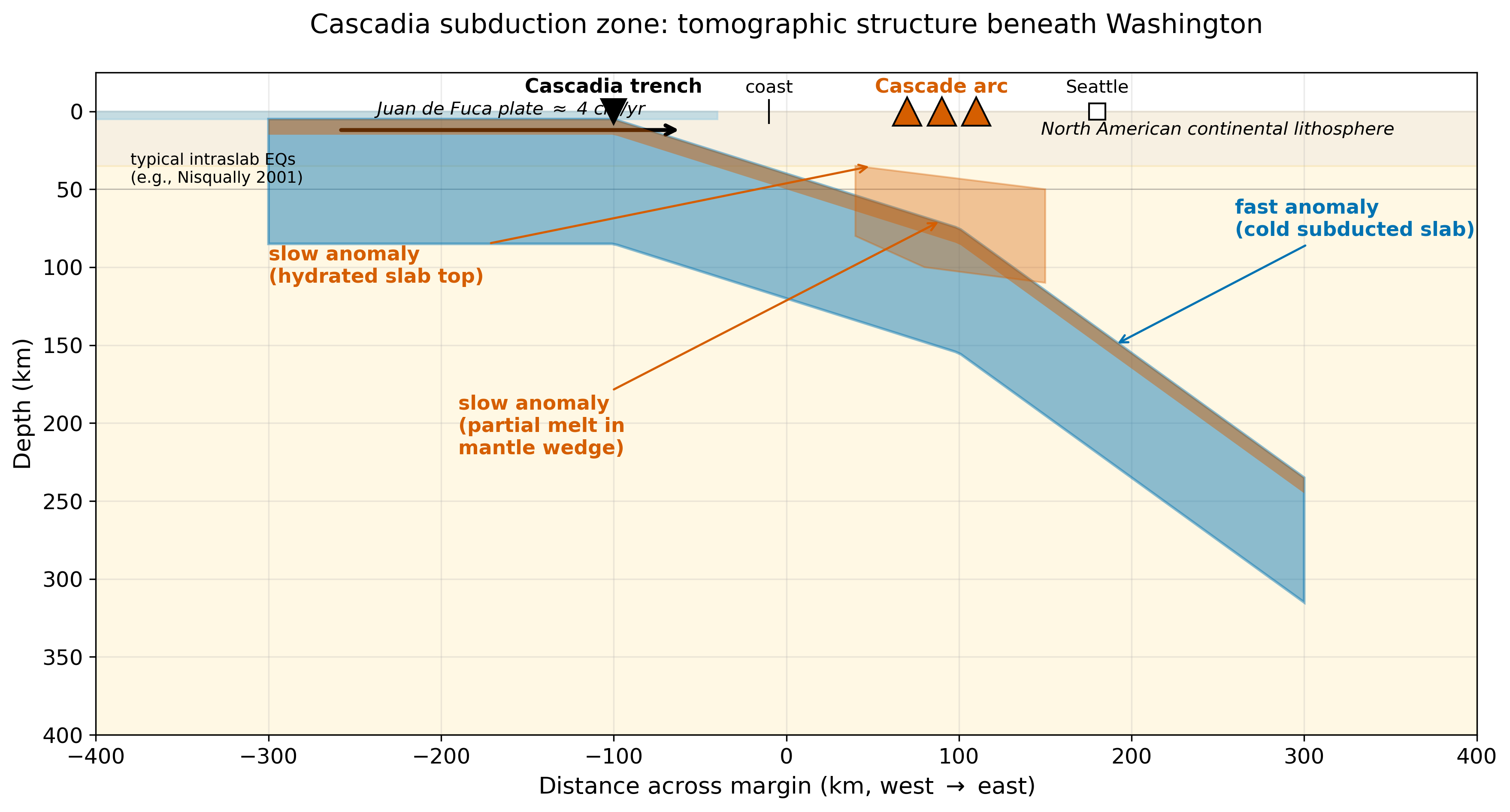
East-west cross-section of the Cascadia subduction zone — Fig. 48 beneath Washington state. The horizontal axis spans from 400 km west of the coast to 400 km east; the vertical axis is depth from 0 at the top to 400 km downward. A blue polygon representing the subducting Juan de Fuca slab descends from the trench at the left with a shallow dip of about 15 degrees near the surface, steepening to about 45 degrees below 100 km depth, and extending to roughly 350 km depth at the right edge. Orange shading on the top surface of the slab indicates a hydrated slab-top low-velocity layer, and an orange wedge-shaped region at 50-110 km depth beneath the Cascade arc represents the mantle wedge partial-melt zone. Symbols at the surface mark, from left to right: the Cascadia trench offshore, the coastline, Seattle (in the Puget Lowland, west of the volcanic arc), and the Cascade arc volcanoes (orange triangles) near the right edge of the profile. A black arrow shows the Juan de Fuca plate moving eastward at about 4 cm/yr. Labels identify the fast (blue) anomaly as the cold subducted slab and the slow (orange) anomalies as the hydrated slab top and the partial-melt mantle wedge. :width: 100%#

The Cascadia subduction zone in tomographic cross-section. The fast blue anomaly is the cold subducted Juan de Fuca slab; the slow orange anomalies are the hydrated slab-top boundary layer and the partial- melt mantle wedge that feeds the Cascade arc. This image, built from thousands of travel-time measurements across EarthScope/Transportable Array stations, is the kind of subsurface picture that this lecture teaches you to make and to critique.

This is what tomography is for. In Lecture 11, we built a spherically symmetric reference Earth from globally averaged travel-time curves. In this lecture we refine the picture: instead of one function \(V(r)\), we solve for \(V(r, \theta, \phi)\) — a three-dimensional map of velocity inside the planet. Geophysically, tomography is what turned the Earth’s mantle from a homogeneous fluid envelope into a visible circulating engine of plate tectonics.

2. The physics: ray cones and the information a single seismogram carries#

The fundamental geometrical observation is that a single travel-time measurement localises a subsurface anomaly only to a narrow cone connecting source to receiver. A fast blob somewhere along the ray path will shorten the travel time; a slow blob will lengthen it; but neither the travel time alone, nor the measurement at a single station, can tell us where along the ray the anomaly sits.

A second earthquake at a different location illuminates the same target along a different cone. The intersection of the two cones localises the anomaly in two dimensions. Many earthquakes and many stations, with many crossing rays, localise it in three. Figure Fig. 49 shows the sequence.

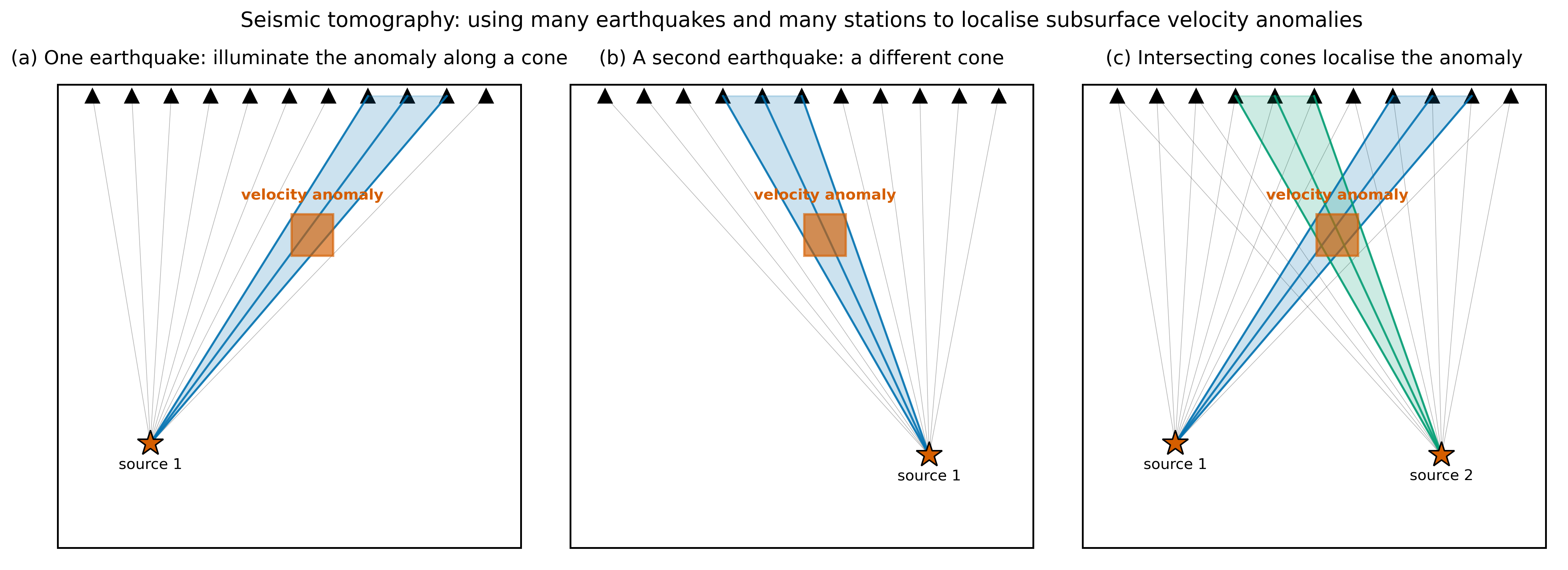
Three side-by-side square panels, each showing a row of — Fig. 49 eleven black triangle station markers across the top and a velocity-anomaly square marked in orange near the centre. In the first panel, an orange star source at the lower left sends thin grey rays to each station; three rays passing through the anomaly are highlighted in thick blue, forming a wedge-shaped cone. In the second panel, an orange star source at the lower right likewise sends rays; the three rays passing through the anomaly are highlighted in thick blue, forming a different-angled cone aimed the other way. In the third panel, both sources are shown; two cones (one blue from left source, one green from right source) intersect at the orange anomaly square, and the overlap of the two cones pinpoints the anomaly location. Each panel is captioned respectively “(a) One earthquake: illuminate the anomaly along a cone,” “(b) A second earthquake: a different cone,” “(c) Intersecting cones localise the anomaly.” :width: 100%#

The geometric core of seismic tomography. A single earthquake illuminates a velocity anomaly along a cone of possible locations. A second earthquake at a different location illuminates a different cone. Their intersection pinpoints the anomaly. Real tomography uses thousands of earthquakes and thousands of stations; the spatial resolution of the final image is set by the geometry of this illumination.

The practical implication is that source-receiver coverage controls resolution. A region that has been crossed by many rays from many azimuths — for example, Japan, California, western Europe — is well imaged. A region crossed by few rays from narrow azimuths — the oceans, Antarctica, the Southern Hemisphere generally — is poorly imaged. This is a fundamental asymmetry of seismic tomography and it shows up in every global image. Whenever a tomographic map is published, the authors also publish a resolution test: a synthetic inversion in which a known pattern (typically a checkerboard of alternating fast and slow anomalies) is forward-modelled through the same ray geometry, corrupted with the same noise, and inverted with the same code. Regions where the checkerboard is recovered are trustworthy; regions where it is smeared or missing are not.

3. The mathematical framework: discretising the forward problem#

To make tomography computable, we discretise the Earth into cells and assume the slowness is constant within each cell. The travel time along a ray then becomes a weighted sum over the cells the ray crosses:

(97)#\[t_k \;=\; \sum_{i=1}^{N} G_{ki}\, s_i,\]

where \(t_k\) is the travel time of the \(k\)-th ray, \(s_i\) is the slowness of the \(i\)-th cell, and \(G_{ki}\) is the path length of ray \(k\) through cell \(i\). In matrix form,

(98)#\[\mathbf{d} = \mathbf{G}\,\mathbf{m},\]

where \(\mathbf{d}\) is the vector of \(M\) observed travel times (the data), \(\mathbf{m}\) is the vector of \(N\) cell slownesses (the model), and \(\mathbf{G}\) is the \(M \times N\) forward operator (a sensitivity matrix) whose entries are the geometric path lengths. The same two symbols — \(\mathbf{G}\) and \(\mathbf{m}\) — recur throughout inverse theory. Memorise them.

Notation

\(\mathbf{d}\): data vector, length \(M\), containing one travel time per observed ray.
\(\mathbf{m}\): model vector, length \(N\), containing one slowness per cell.
\(\mathbf{G}\): sensitivity matrix, \(M \times N\), with \(G_{ki}\) equal to the path length (km) of ray \(k\) through cell \(i\). Most entries are zero because most rays do not cross most cells.
Scalar quantities: \(M\) = number of rays; \(N\) = number of cells.

The smallest possible example is a \(2 \times 2\) grid of cells with two horizontal rays and two vertical rays. Figure Fig. 50 (a) shows the geometry; the system of equations it encodes is

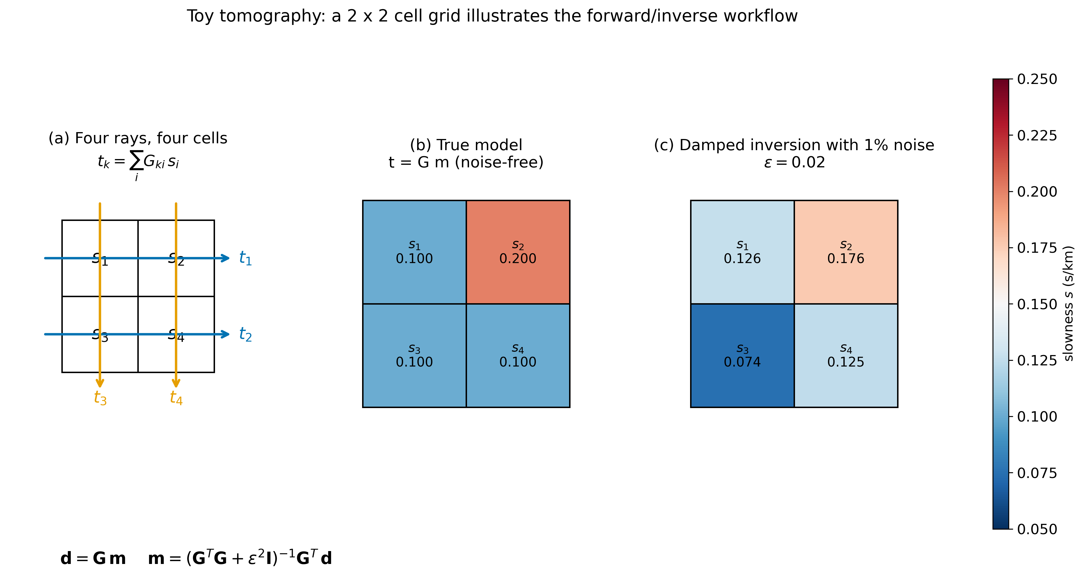
(99)#\[\begin{split}\begin{aligned} t_1 &= s_1 h + s_2 h \\ t_2 &= s_3 h + s_4 h \\ t_3 &= s_1 h + s_3 h \\ t_4 &= s_2 h + s_4 h \end{aligned} \quad\Longleftrightarrow\quad \underbrace{\begin{pmatrix} t_1\\ t_2\\ t_3\\ t_4 \end{pmatrix}}_{\mathbf{d}} \;=\; \underbrace{\begin{pmatrix} h & h & 0 & 0\\ 0 & 0 & h & h\\ h & 0 & h & 0\\ 0 & h & 0 & h\end{pmatrix}}_{\mathbf{G}} \underbrace{\begin{pmatrix} s_1\\ s_2\\ s_3\\ s_4 \end{pmatrix}}_{\mathbf{m}}.\end{split}\]

Three-panel figure. Panel (a) shows a two-by-two grid of four — Fig. 50 cells labelled s1 through s4 in black outlines, with two horizontal blue arrows labelled t1 and t2 passing through the top and bottom rows and two vertical orange arrows labelled t3 and t4 passing through the left and right columns. Panel (b) shows the same grid coloured by a blue-to-red colormap representing slowness values: three cells have slowness 0.100 s/km (light blue), one cell (top right, s2) has slowness 0.200 s/km (salmon). Panel (c) shows the grid after damped inversion with 1 percent noise; cells now have slownesses 0.126, 0.176, 0.074, and 0.125 respectively, the anomaly is still located in the top right but the other three cells show recovery errors from the noise and damping. A vertical colorbar on the right runs from blue (0.05 s/km) to red (0.25 s/km). Below the panels, the matrix equations d equals G m and m equals parenthesis G-transpose G plus epsilon squared identity parenthesis inverse G-transpose d are written. :width: 100%#

The simplest possible seismic tomography problem. Panel (a) shows the geometry: four cells, four rays. Panel (b) shows a “true” model with one slow cell (salmon, top right). Panel (c) shows the damped inversion of noisy data, where the slow anomaly is correctly localised but the amplitude is spread into neighbouring cells — a pedagogically honest demonstration of how damping trades resolution for stability.

Even this toy system has a subtle flaw. The matrix \(\mathbf{G}\) is rank-3, not rank-4: any uniform change to all four slownesses satisfies all four travel-time equations equally well. This is a null space of the forward operator — a direction in model space that the data cannot see. Every real tomographic inversion has such null spaces, and the job of regularisation is to decide which model the inversion returns when the data are indifferent.

3b. Snell’s law bends the rays — and that makes \(\mathbf{G}\) non-linear#

The derivation above assumes the path of each ray through the cells is known and fixed: \(G_{ki}\) is simply the geometric length of a straight line (or a pre-computed reference-model path) through cell \(i\). In reality, rays obey Snell’s law at every interface: whenever velocity changes, the ray direction changes to conserve the ray parameter \(p = \sin i / V\). This means the actual path — and therefore every entry \(G_{ki}\) — depends on the very velocity model \(\mathbf{m}\) we are trying to recover. The forward problem is non-linear:

(100)#\[\mathbf{d} = \mathbf{F}(\mathbf{m}),\]

where \(\mathbf{F}\) is the full (non-linear) forward operator that computes travel times by tracing rays through the model.

Standard fix — linearise around a reference model. Let \(\mathbf{m}_0\) be a smooth 1-D reference (e.g. AK135), and let \(\delta\mathbf{m} = \mathbf{m} - \mathbf{m}_0\) be the perturbation we seek. Expanding \(\mathbf{F}\) to first order (the Born approximation for ray theory),

(101)#\[\delta\mathbf{d} \;\approx\; \mathbf{G}(\mathbf{m}_0)\,\delta\mathbf{m},\]

where \(\delta\mathbf{d} = \mathbf{d}_\text{obs} - \mathbf{F}(\mathbf{m}_0)\) are the travel-time residuals and \(\mathbf{G}(\mathbf{m}_0)\) is the sensitivity matrix evaluated on the reference-model ray paths. The system is now linear in \(\delta\mathbf{m}\) and can be treated with standard least squares.

Iterative solution. Because Eq. (101) is only approximate, we iterate:

Compute reference-model ray paths and residuals \(\delta\mathbf{d}^{(0)}\).
Invert for \(\delta\mathbf{m}\) using damped least squares (Eq. (103)).
Update the model: \(\mathbf{m}_1 = \mathbf{m}_0 + \delta\mathbf{m}\).
Retrace rays through \(\mathbf{m}_1\), compute new residuals, repeat.

This loop converges in a few iterations for well-sampled problems. For poorly-sampled problems the loop can diverge or stagnate, and one must rely on smoothing to stabilise it.

Full-waveform inversion (FWI) goes further still. Rather than collapsing a seismogram to a single travel-time number, FWI minimises the misfit between the entire observed waveform and a simulated waveform computed by solving the 3-D elastic wave equation numerically (SPECFEM3D). The sensitivity matrix is replaced by adjoint kernels — volumetric sensitivity maps computed from pairs of forward and adjoint simulations. This approach captures finite- frequency effects (curved sensitivity lobes, “banana-doughnut” kernels) that ray theory ignores, and it doubles the spatial resolution achievable from the same dataset.

The non-linear chain in one sentence

Ray paths depend on velocity → \(\mathbf{G}\) depends on \(\mathbf{m}\) → the forward problem is non-linear → we linearise around a reference model and iterate, or replace ray theory with a full numerical wave simulation.

4. The inverse problem: least squares and why it needs help#

If \(\mathbf{G}\) were square and invertible, the model would be recovered by direct inversion: \(\mathbf{m} = \mathbf{G}^{-1}\mathbf{d}\). It never is. Typically there are far more cells than rays, or the ray coverage is uneven so that some rays are redundant, or small measurement errors in \(\mathbf{d}\) produce huge changes in \(\mathbf{m}\). The standard remedy is ordinary least squares, which finds the model that minimises the sum of squared data residuals:

(102)#\[\hat{\mathbf{m}}_{\mathrm{OLS}} \;=\; \arg\min_{\mathbf{m}} \|\mathbf{d} - \mathbf{G}\mathbf{m}\|_2^2 \;=\; (\mathbf{G}^{T}\mathbf{G})^{-1}\mathbf{G}^{T}\mathbf{d}.\]

The problem is that \(\mathbf{G}^{T}\mathbf{G}\) is often singular or near-singular, and inverting it produces a solution dominated by noise. Damped least squares adds a small positive term to the diagonal of \(\mathbf{G}^{T}\mathbf{G}\) before inverting:

(103)#\[\hat{\mathbf{m}}_{\mathrm{DLS}} \;=\; (\mathbf{G}^{T}\mathbf{G} + \varepsilon^{2}\mathbf{I})^{-1}\mathbf{G}^{T}\mathbf{d}.\]

Damping penalises large model perturbations. The result is a solution whose amplitude is biased toward zero (toward the reference model) but whose spatial pattern is stable against small data errors. The penalty scalar \(\varepsilon^2\) controls the trade-off: small \(\varepsilon^2\) gives high resolution but high noise sensitivity; large \(\varepsilon^2\) gives a heavily smoothed, low-amplitude image. Choosing \(\varepsilon^2\) is an art, usually informed by an L-curve analysis (plotting data misfit versus model norm across a range of \(\varepsilon^2\) and selecting the corner).

Key Equation — damped least squares

\[ \hat{\mathbf{m}} \;=\; \bigl(\mathbf{G}^{T}\mathbf{G} + \varepsilon^{2}\mathbf{I}\bigr)^{-1}\mathbf{G}^{T}\mathbf{d}. \]

This single line summarises the workhorse of seismic tomography. Every global mantle model published in the last thirty years is some variant of it: weighted least squares (which uses a data-covariance weighting \(\mathbf{W}_d\)), Tikhonov regularisation (which penalises spatial roughness instead of amplitude), or iterative non-linear generalisations. The core idea is always the same — trade a little resolution for a lot of stability.

Two philosophical cautions are worth internalising now. First, the inverse problem has no unique solution. A family of models fits the data equally well within error; regularisation selects one. The model we plot is a choice. Second, the resolution is not uniform. Near the edges of the array, or in depth ranges where few rays bottom, the recovered anomaly is smeared and attenuated. A responsible tomographer always reports resolution tests alongside the result.

Reasoning sketch — choosing \(\varepsilon^2\) via the L-curve

The damping parameter \(\varepsilon^2\) is not given by the data — it is a modeller’s choice that trades two competing goods:

Data misfit \(\|\mathbf{d} - \mathbf{G}\hat{\mathbf{m}}\|_2\): small \(\varepsilon^2\) → low misfit (the model fits the data, including the noise).
Model norm \(\|\hat{\mathbf{m}}\|_2\): small \(\varepsilon^2\) → large model amplitudes (resolved features and noise alike are amplified).

Plot one against the other across a range of \(\varepsilon^2\) and the points fall on an L-shaped curve: a near-vertical branch where reducing \(\varepsilon^2\) buys huge model norm for negligible misfit improvement (overfitting noise), a near-horizontal branch where increasing \(\varepsilon^2\) throws away resolution for negligible norm gain (over-smoothing), and a corner where the two trade off fairly. The corner is conventionally chosen.

Reasoning question for office hours. If a colleague says “I just used \(\varepsilon^2 = 0.01\) because that’s the default,” what follow-up question do you ask? What single figure in the paper would let you check whether the choice is defensible?

5. Worked interpretation: reading a mantle tomographic image#

The global tomographic image, built by combining millions of travel-time residuals from all the permanent seismic networks and several decades of temporary deployments, looks like Figure Fig. 51. The basic features to recognise are:

Blue (fast) linear features descending through the upper mantle and into the lower mantle beneath subduction zones. These are cold, dense slabs sinking at \(\sim\) cm/yr. Some slabs stagnate at the 660-km discontinuity (western Pacific), others punch through and descend to the core-mantle boundary (Farallon slab beneath North America).
Red (slow) columnar features rising from the lower mantle under hotspot volcanoes. These are interpreted as thermo-chemical plumes; the Yellowstone, Hawaii, Iceland, and Afar plumes are the best documented. Whether all plumes root at the CMB is actively debated.
Large low-shear-velocity provinces (LLSVPs) at the base of the mantle beneath the central Pacific and Africa. These cover about 25% of the CMB and extend a few hundred kilometres upward. Their origin — compositional, thermal, or both — is unresolved.
Ultra-low velocity zones (ULVZs): 10- to 50-km-thick patches at the CMB with extreme velocity reductions (−30% for \(V_S\)). Thought to be partial melts or iron-enriched.
The D″ layer, a few-hundred-kilometre-thick discontinuity just above the CMB, seen in ScS precursors and thought to be a post-perovskite phase transition.

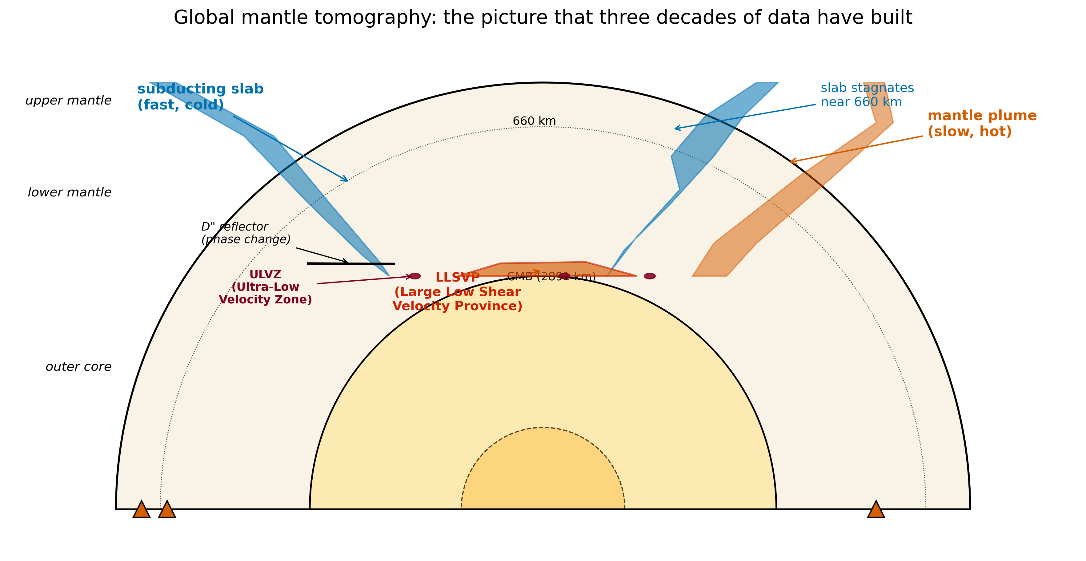
Pole-to-pole semicircular cross-section of Earth showing three — Fig. 51 layers: a thin surface ring, a shaded mantle region, and an inner core region. Two blue angular slab shapes descend from the surface on opposite sides: a left-side slab extending from near the surface to the core-mantle boundary at 2891 km depth, and a right-side slab that curves and flattens at about 660 km depth before descending further. An orange plume-shaped feature rises on the right from the core-mantle boundary to the surface. At the base of the mantle, a wide orange region just above the CMB represents a large low-shear velocity province, labelled LLSVP. Small dark-red patches on the CMB are labelled ULVZ (ultra-low velocity zone). A short black irregular line above the CMB is labelled D double-prime reflector. Orange triangles at the surface mark volcanic arcs on both sides. Text labels identify “subducting slab (fast, cold)”, “slab stagnates near 660 km”, “mantle plume (slow, hot)”, “LLSVP”, “ULVZ”, and “D double-prime reflector”. :width: 100%#

The global mantle as mapped by decades of seismic tomography. Subducting slabs appear as fast, cold features descending into the lower mantle. Mantle plumes rise as slow, hot columnar features. At the base of the mantle, large low-shear-velocity provinces (LLSVPs) and ultra-low velocity zones (ULVZs) mark the chemical and thermal heterogeneity of the lowermost mantle. The D″ discontinuity just above the CMB reflects a pressure-induced phase transition. This picture is not the output of a single inversion — it is the consensus view emerging from dozens of independent tomographic studies over thirty years.

The Cascadia slab of Section 1 fits this global picture as a typical subduction signature: fast, cold, 80 km thick, dipping eastward. Its resolved extent to \(\sim\) 350 km depth reflects both the real geometry and the limits of current ray coverage beneath the PNW. Resolving the deeper slab structure requires PKP-like teleseisms, dense broadband networks (EarthScope Transportable Array passed through Washington in 2007–2009), and ambient-noise surface-wave tomography.

A worked example from the published literature: the Farallon slab#

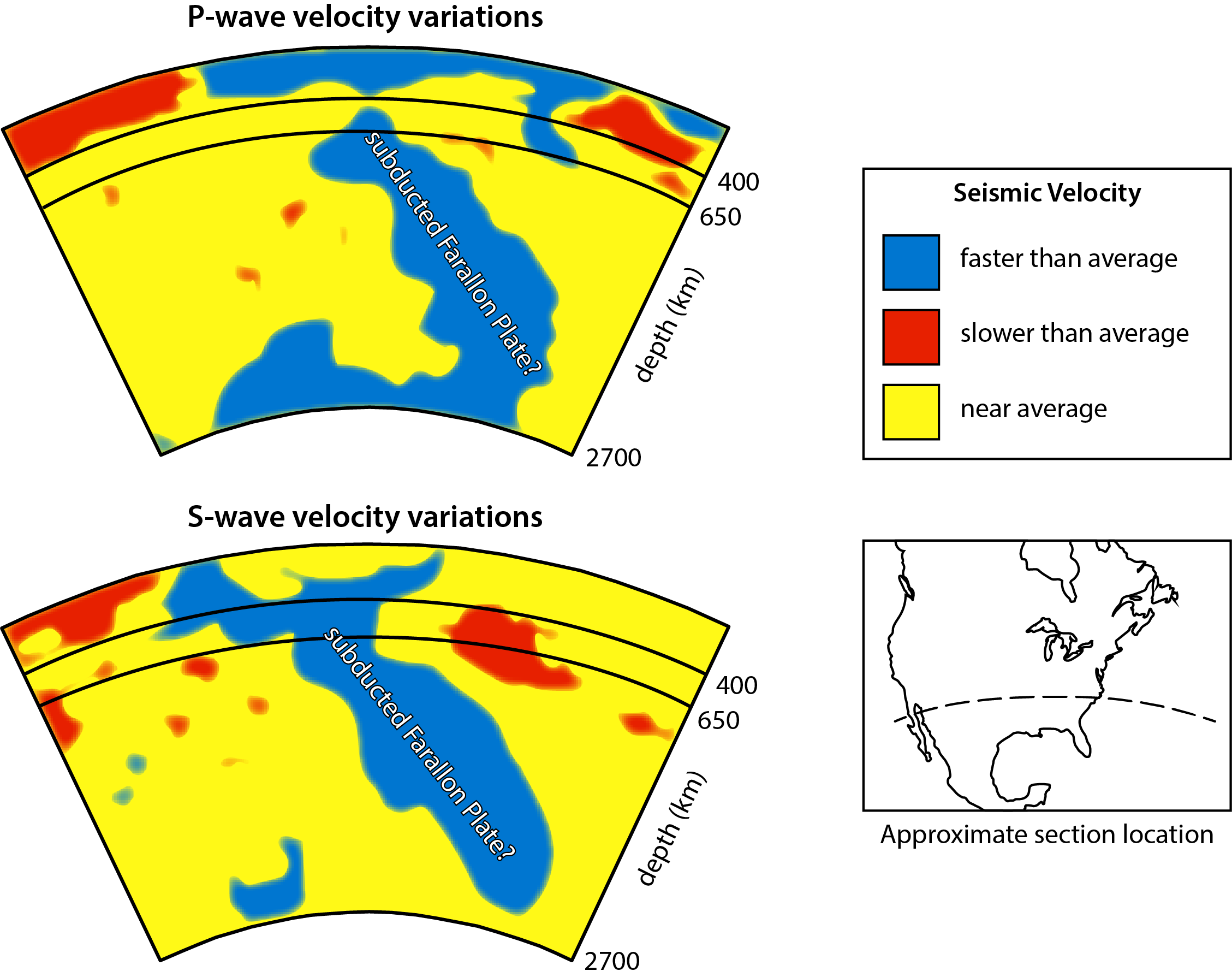
Cross-section of the Earth's mantle from the surface to the — Fig. 52 core-mantle boundary at 2891 km depth, showing P-wave (left half) and S-wave (right half) velocity perturbations beneath southern North America. A continuous fast (blue) tabular feature dips from the western surface beneath North America, flattens broadly between about 660 and 1500 km depth, and then descends more steeply into the lowermost mantle. Slow (red) regions appear in the upper-mantle asthenosphere and in patches of the lowermost mantle. The fast feature is labelled the Farallon slab; the lowermost-mantle slow patch corresponds to the African / Pacific large low-shear-velocity province. :width: 95%#

**A real published tomographic cross-section: the Farallon slab beneath North America.** The image (CC BY-SA 4.0; Wikimedia Commons user *Oilfieldvegetarian* after Grand, van der Hilst & Widiyantoro 1997, *GSA Today* 7(4), 1–7) shows P-wave velocity perturbations on the left and S-wave perturbations on the right. The slab is the fast (blue) tabular feature that subducted under western North America in the Mesozoic, stalled in the mid-mantle, and sinks today toward the core–mantle boundary. Compare it to the schematic in Fig. 51: the published image shows the same kinematic features, but with real ray-coverage gaps, smearing along illumination direction, and amplitude reductions where damping dominates. **Reading exercise:** identify (i) the upper-mantle low-velocity zone, (ii) the slab segment that has stalled near 660 km, and (iii) at least one region where the recovered amplitude is suspect because the illumination is one-sided.

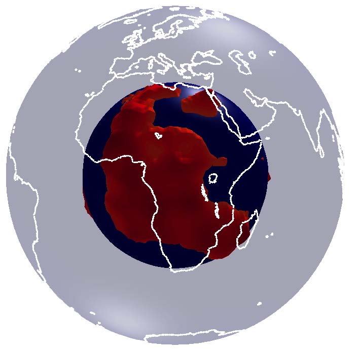
Three-dimensional cartoon of Earth's lower mantle viewed from — Fig. 53 the south Atlantic side, showing the African large low-shear-velocity province (LLSVP) as a translucent red dome rising from the core-mantle boundary into the lower mantle beneath southern Africa and the southwest Indian Ocean. The CMB is shown as a smooth orange shell at the base; the dome’s outline is irregular but coherent. :width: 60%#

**The African LLSVP — a deep-mantle structure inferred from S-wave tomography.** Cartoon by Sanne Cottaar (CC BY-SA 3.0; Wikimedia Commons), based on her published cluster analysis of multiple shear-wave tomographic models Cottaar and Lekic [2016]. The two LLSVPs (the African one shown here, and a second beneath the central Pacific) together cover roughly a quarter of the core-mantle boundary, are about 1000 km tall, and are reproducibly recovered by independent inversions. Whether they are dominantly thermal piles or thermo-chemical reservoirs remains an open research question — and the answer matters for whether mantle plumes anchor at LLSVP edges, where some hotspots (Iceland, Hawaii, Tristan) appear to root.

A small literature gallery — open-access papers per section

Paper figures are protected by their journals’ licences. Where a figure is not directly embeddable here we link to its open-access source so you can read it in context. Verify each DOI yourself.

Section	Open-access paper	What its figures show
§2 ray cones, §7 resolution	Rawlinson et al. [2010] Phys. Earth Planet. Inter. 178 (open-access PDF widely available) — Seismic tomography: a window into deep Earth	Comprehensive review with worked examples of ray-density maps, checkerboard tests, and trade-off curves. Best single reading for §7.
§3 forward problem, §4 inverse	Aster et al. [2018] Parameter Estimation and Inverse Problems (UW Libraries)	Schematic of \(\mathbf{G}\) for travel-time tomography; L-curve worked examples.
§5 LLSVPs, lower-mantle structure	Cottaar & Lekić (2016) Geophys. J. Int. 207, 1122–1136 — https://doi.org/10.1093/gji/ggw324 (Open Access)	The LLSVP cluster analysis behind Fig. 53; Figure 4 is a clear depth-by-depth map of consensus structure.
§5 deep mantle plumes	Koppers et al. (2021) Nat. Rev. Earth Environ. 2, 382–401 — https://doi.org/10.1038/s43017-021-00168-6	Fig. 2 compares plume locations across multiple modern tomographic models — useful when judging which features are “robust”.
§6 ambient-noise / joint	Wang, Lin & Ward (2019) Geophys. J. Int. 217, 1668–1680 — https://doi.org/10.1093/gji/ggz109 (OA)	Cascadia ambient-noise tomography using dense linear arrays; their Fig. 5 is a textbook example of a joint shallow \(V_S\) image.
§7 resolution / checkerboard	Rawlinson & Spakman (2016) Tectonophysics 670, 1–8 — On the use of sensitivity tests in seismic tomography	Full discussion (with examples) of the limits of checkerboard tests as resolution proxies — the paper that warns against trusting them as the only diagnostic.
§10 FWI	Lei et al. (2020, GLAD-M25) Geophys. J. Int. 223, 1–21 — https://doi.org/10.1093/gji/ggaa253 (OA)	Fig. 6 (mantle cross-sections) and Fig. 11 (resolution tests) of GLAD-M25.
§10 ML / phase picking	Woollam et al. (2022, SeisBench) Seismol. Res. Lett. 93, 1695–1709 — https://doi.org/10.1785/0220210324 (OA)	Fig. 1 of the SeisBench architecture; benchmarks across networks.
§10 Mars / planetary	Stähler et al. (2021) Science 373, 443–448 — https://doi.org/10.1126/science.abi7730	Fig. 1 (Mars seismogram + ray paths) and Fig. 3 (recovered Martian core radius) — the same inverse-problem framework on a different planet.

These are the figures we asked you to read alongside the lecture. Whenever a tomographic image is reproduced in a textbook or a slide deck, trace it back to a primary paper and inspect the resolution test the authors actually published.

6. Combining body-wave and surface-wave tomography#

Body waves and surface waves probe the Earth in fundamentally different ways, and a tomographic image built from one alone has predictable blind spots that the other can fill. Modern tomography treats the two as complementary observables that should be inverted together whenever possible.

Body waves (P, S, PcP, PKP, …) carry sensitivity along narrow ray paths that turn deep in the mantle. They give good lateral resolution in the lower mantle but only where rays actually pass through. Beneath an aseismic, sparsely-instrumented region (most of the oceans, most of the Southern Hemisphere), no body-wave ray ever turns there, and no body-wave inversion can constrain the structure.

Surface waves (Rayleigh, Love) propagate along the Earth’s surface with a depth sensitivity that is set by their period: longer periods sample deeper. Their sensitivity is a smooth, broad depth kernel that integrates over a few hundred kilometres vertically, so depth resolution is poor — but they sample every great-circle path between any pair of stations, and (via ambient-noise cross-correlation) can be obtained without earthquakes. Surface waves therefore give good shallow lateral coverage even where body-wave coverage is sparse, but cannot resolve sharp vertical contrasts.

The two are perfectly complementary: body waves give vertical resolution where rays pass; surface waves give horizontal coverage everywhere shallow.

How a joint inversion is built#

Stack the body-wave and surface-wave equations into a single linear system:

(104)#\[\begin{split}\begin{pmatrix} \mathbf{W}_b\,\mathbf{d}_b \\ \mathbf{W}_s\,\mathbf{d}_s \end{pmatrix} \;=\; \begin{pmatrix} \mathbf{W}_b\,\mathbf{G}_b \\ \mathbf{W}_s\,\mathbf{G}_s \end{pmatrix} \,\mathbf{m},\end{split}\]

where \(\mathbf{d}_b\) are body-wave travel-time residuals, \(\mathbf{d}_s\) are surface-wave dispersion measurements (phase or group velocity vs. period at each path), and \(\mathbf{W}_b\), \(\mathbf{W}_s\) are diagonal weighting matrices that scale each block by its data-uncertainty and balance the relative contribution of the two datasets. The combined system is then inverted with damped least squares (Eq. (103)) exactly as before. Choosing the relative weighting is itself a regularisation choice; common practice is to vary the body/surface weight ratio across an order of magnitude and verify the recovered model is stable.

Surface-wave dispersion enters \(\mathbf{G}_s\) through depth sensitivity kernels \(K(z; T)\) that say how strongly a phase velocity at period \(T\) depends on the shear-velocity profile at each depth. The kernels are smooth bumps centred near \(z \sim T \cdot V_S\) (the rule of thumb: a 30-second Rayleigh wave samples roughly the upper 80–100 km). Inverting many periods together unstacks the depth integral and yields a \(V_S(z)\) profile at every surface point.

Why the combination wins in Cascadia#

In the Pacific Northwest, the EarthScope Transportable Array (TA) provided body-wave coverage of the upper-mantle slab geometry, while ambient-noise tomography from PNSN and TA stations provided high-resolution shallow \(V_S\) images of the forearc, back-arc, and mantle wedge without needing earthquakes. Joint inversions (Schmandt and Humphreys 2010, then iteratively refined by many groups) leverage both: the body waves anchor the slab below 100 km; the surface waves resolve the crust and uppermost mantle. Neither dataset alone gives the full picture in Figure Fig. 78.

A practical observation

A modern Cascadia tomography paper almost always shows: (i) a body-wave \(\delta V_P\) image to deep mantle, (ii) an ambient-noise \(V_S\) image for the upper 50 km, and (iii) a joint \(V_S\) image that splices them across 50–150 km depth. The transitions between datasets are the places to scrutinise critically — different sensitivity kernels can produce different amplitudes for the same feature.

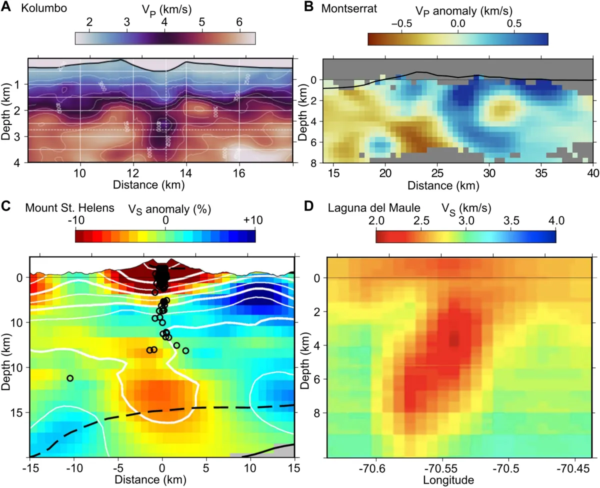
Four-panel composite showing real joint-inversion tomographic — Fig. 54 results from four volcanic systems—Kolumbo (full-waveform inversion of marine streamer data), Montserrat (joint travel-time and gravity inversion), Mount St Helens (joint local-earthquake and ambient-noise surface-wave tomography), and Laguna del Maule (ambient-noise surface wave tomography). Each panel shows a vertical cross-section of P- or S-wave velocity anomaly with a low-velocity body interpreted as magma or crystal mush at depths of a few kilometres beneath the edifice. :width: 95%#

**Four real joint-inversion images of magmatic systems.** Reproduced from Figure 8 of Paulatto *et al.* [2022] under CC BY 4.0. Each panel combines a different mix of observables: (a) full-waveform inversion (FWI) of marine streamer data at Kolumbo; (b) joint travel-time + gravity inversion at Montserrat; (c) joint local-earthquake + ambient-noise surface-wave tomography at Mount St Helens; (d) ambient noise surface-wave tomography at Laguna del Maule. **Reading exercise (geophysical reasoning):** the four methods differ in the depth range they constrain best and in their vertical vs. lateral resolution. Identify which panel best resolves a *vertically extensive* low-velocity body (a tall mush column rather than a thin sill) and defend your choice in three sentences, citing the underlying observable each method depends on.

7. Estimating resolution: where can we trust the image?#

Every tomographic image lives or dies on its resolution map — the spatial distribution of how well, or how poorly, the inversion can constrain the model. A region of an image where the inversion cannot constrain the model and the inversion drifts toward whatever the regularisation prefers (often zero, or smoothness) is not the same as a region where the inversion finds genuinely zero anomaly. Telling these apart is the most important step in interpreting a tomographic image responsibly.

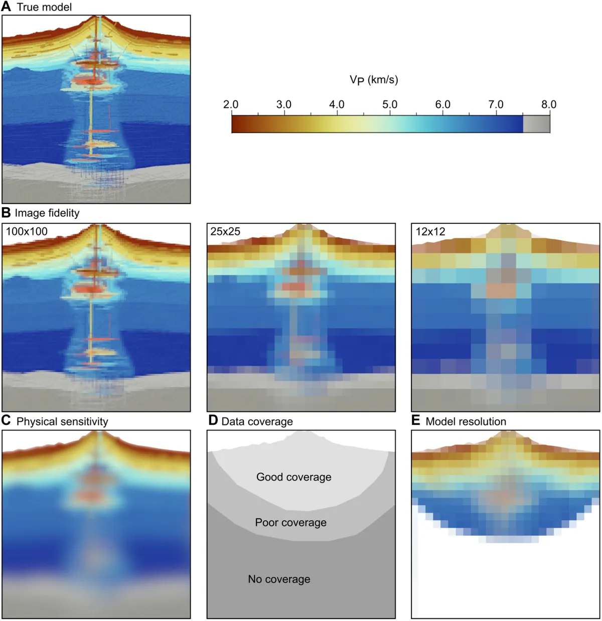
Multi-panel synthetic recovery test. The top row shows the true — Fig. 55 velocity model (an idealised volcano with a low-velocity magma body at depth). Subsequent rows isolate four distinct effects on the recovered image—image fidelity (the choice of imaging method), physical sensitivity (the wavefield’s intrinsic ability to sense the target), data coverage (the source-receiver geometry), and model resolution (the regularisation and parametrisation). Each row shows how that single effect, in isolation, blurs or biases the recovered low-velocity body. :width: 90%#

**The four effects that limit any tomographic image.** Reproduced from Figure 2 of Paulatto *et al.* [2022] under CC BY 4.0. The same idealised target (a magma body) is recovered under four separate degradations: imaging-method fidelity, physical sensitivity, data coverage, and regularisation/model resolution. Together these set the ceiling on what *any* tomographic experiment can recover. **Reading exercise (geophysical reasoning):** suppose you want to image a 5-km-wide low-velocity body at 30 km depth using a 50-station local network and local earthquakes. Which of the four panels depicts the *binding constraint* for your survey — the one effect that will dominate the blurring of your final image? Justify in three sentences, then state one thing you could change about the experiment to relax that constraint.

The two ingredients of poor resolution#

Sparse sources. Earthquakes occur almost exclusively at plate boundaries — subduction zones, mid-ocean ridges, transforms. Source-rich regions (Japan, Aleutians, Andes, Indonesia, Mediterranean) provide rays from many azimuths. Source-poor regions (most of the ocean basins, intraplate continents, Antarctica) provide rays from one or two azimuths at most.
Sparse stations. Permanent broadband stations cluster in wealthy, populated continents. Oceans, deserts, polar regions carry few stations. Temporary deployments (USArray, AlpArray, AfricaArray) have radically improved coverage in their target regions for ~5-year windows.

The product of these two distributions — the ray density in each cell — is the first-order proxy for resolution. Cells crossed by many rays from many azimuths are well constrained; cells crossed by few rays, or by parallel rays, are not.

Ray density maps as a quick-look resolution proxy#

The fastest resolution diagnostic, computed at essentially zero cost once \(\mathbf{G}\) is built, is the ray-density map: count the number of non-zero entries in each column of \(\mathbf{G}\), or equivalently sum the path lengths through each cell. This is displayed alongside the tomographic image and immediately reveals which features sit in well-illuminated regions versus illumination shadows. A more directional version is the azimuthal coverage, which counts not just the number of rays but how uniformly their azimuths span 360°: a cell crossed by 1000 rays all in a north-south direction is not well resolved laterally.

The diagonal of the resolution matrix \(\mathbf{R}\)#

The formal answer is the resolution matrix \(\mathbf{R}\), defined by composing the linearised inverse and forward operators:

(105)#\[\hat{\mathbf{m}} = \mathbf{R}\,\mathbf{m}_\text{true}, \qquad \mathbf{R} = (\mathbf{G}^{T}\mathbf{G} + \varepsilon^{2}\mathbf{I})^{-1}\mathbf{G}^{T}\mathbf{G}.\]

If \(\mathbf{R}\) were the identity matrix the inversion would recover the true model exactly. In practice it is not. The diagonal \(R_{ii}\) measures how much of the true value of cell \(i\) ends up in the recovered model: \(R_{ii} = 1\) means perfect recovery; \(R_{ii} \ll 1\) means the inversion is recovering only a small fraction (the rest is suppressed by damping or smeared into neighbours). The off-diagonal entries \(R_{ij}\) measure smearing between cells. A row of \(\mathbf{R}\) is the point-spread function of the inversion at one cell — the image that the inversion would return for a delta-function input there.

For large problems \(\mathbf{R}\) is impractical to form explicitly, but its diagonal can be approximated stochastically (probing with random vectors).

Synthetic tests: checkerboard, spike, and “input model” tests#

The community standard for empirical resolution assessment is the checkerboard test:

Build a synthetic “true” model — a regular grid of alternating fast and slow anomalies of known size and amplitude.
Forward-model it through the same \(\mathbf{G}\) used for the real inversion: \(\mathbf{d}_\text{syn} = \mathbf{G}\,\mathbf{m}_\text{cb}\).
Add realistic noise to \(\mathbf{d}_\text{syn}\).
Invert with the same regularisation \(\varepsilon^2\) and workflow.
Compare the recovered checkerboard to the input. Where the pattern is faithfully recovered, the inversion has good resolution at that scale. Where the pattern is smeared, blurred, or rotated, the inversion is unreliable at that scale.

Repeating the test at multiple checkerboard wavelengths gives a scale-dependent resolution map: a region might recover 200-km features but not 50-km features. Spike tests (a single isolated anomaly) and input-model tests (a synthetic that mimics the recovered model) probe different aspects of the same question.

Warning

Checkerboard tests only assess the resolution of the linearised operator \(\mathbf{G}\) at the chosen damping; they do not validate the choice of parametrisation, the linearisation itself, or the adequacy of ray theory. A checkerboard test that “passes” can still miss systematic errors.

Bayesian / probabilistic resolution#

Modern probabilistic tomography (HMC, variational inference) replaces the single regularised solution with a posterior distribution over models. The standard deviation of the posterior at each cell is a directly interpretable, dimensional uncertainty estimate: “the \(V_P\) anomaly at 150 km depth is \(-1.2 \pm 0.4 \%\).” This is the gold standard of resolution reporting and is becoming increasingly common as compute costs fall.

The four-question reading list for any tomographic image

When you read a published tomographic image, ask:

Where are the sources and where are the stations? A ray density or hit-count map should accompany the image.
What checkerboard test was performed and at what scale? The recovered checkerboard should be shown alongside the model.
What damping was used and how was it chosen? An L-curve or trade-off curve should justify the value.
Are uncertainty estimates reported? Posterior standard deviations or model bootstrap variability beat a single regularised model.

A paper that fails to address any of these is incomplete, and the amplitude of any anomaly it reports must be taken as a lower bound at best.

8. Seismic vs. medical tomography: the same mathematics, different geometry#

Computed tomography (CT) scans of the human body and seismic tomography of the mantle are the same inverse problem mathematically. The forward operator \(\mathbf{G}\) in both cases maps a scalar field (X-ray absorption coefficient in medicine, slowness in seismology) to a set of line integrals (X-ray attenuation through tissue, travel time through rock). The crucial difference is the geometry of the sources. In a hospital, the X-ray tube rotates around the patient, illuminating every angle uniformly. In global seismology, the “sources” are earthquakes, located almost exclusively on plate boundaries, which provide a geographically skewed illumination. This is why seismic tomography is a much harder inverse problem than medical CT — not because the physics is more complicated, but because the geometry is worse.

Ambient-noise tomography (Lin et al. 2008, Shapiro et al. 2005) has recently softened this limitation by treating every station as a virtual source. The cross-correlation of continuous ambient seismic noise between two stations converges to a proxy of the Green’s function between them, allowing travel-time tomography without earthquakes. This method has revolutionised regional crustal imaging in the PNW and elsewhere.

9. Connecting to Cascadia: why seeing the slab matters#

The tomographic image of the Juan de Fuca slab in Figure Fig. 78 is not a curiosity. It carries direct implications for PNW seismic hazard.

The shape and steepness of the subducted slab determine the width of the locked megathrust interface, which in turn controls the maximum magnitude of the next Cascadia earthquake. Bodmer et al. (2018) showed that along-strike variations in slab buoyancy correlate with segmentation of the megathrust.
The slab-top low-velocity layer (hydrated, serpentinised) sits along the plate interface and modulates the occurrence of slow slip events — the “episodic tremor and slip” (ETS) phenomenon observed by PNSN stations roughly every 14 months beneath the Olympic Peninsula (Rogers and Dragert 2003).
The mantle-wedge melt zone is what supplies the Cascade arc. Its volume and depth, constrained by tomography, govern the long-term volcanic hazard from Mount Rainier, Mount St Helens, and the rest of the arc.

Every tomographic picture is also a hazard-assessment tool. That is one of many reasons the Pacific Northwest Seismic Network maintains broadband stations across the region, and why EarthScope funded the Transportable Array to sweep east-to-west across the continent.

10. Research Horizon#

The field has moved rapidly from travel-time ray tomography to full-waveform inversion, from human phase pickers to neural networks, and from single-data-type to joint inversions. Below is a snapshot of the frontier as of 2021–2026.

Travel-time → full-waveform inversion#

Global adjoint tomography. The GLAD-M25 model (Lei et al. 2020; https://doi.org/10.1093/gji/ggaa253) demonstrated that spectral-element-based FWI with adjoint kernels (SPECFEM3D_GLOBE) roughly doubles the spatial resolution of classical travel-time tomography at the global scale. Subsequent iterations by the same group (Bozdağ, Peter, Tromp et al.) have extended the approach to higher frequency and larger earthquake datasets; see the review in Tromp 2019 (Nature Reviews Earth & Environment, https://doi.org/10.1038/s43017-019-0003-8) for full context.
Finite-frequency and banana-doughnut kernels. Dahlen et al. (2000) and Tromp et al. (2005) showed that at finite frequency the sensitivity of a travel-time measurement is zero on the geometric ray and peaks in a doughnut-shaped region around it — completely unlike the delta-function sensitivity assumed in ray theory. Modern tomography uses adjoint kernels that correctly represent this, at the cost of one forward + one adjoint simulation per measurement.
Multiscale and collaborative FWI. Fichtner and colleagues (ETH Zurich / ORFEUS) have extended FWI to exploit the entire seismic wavefield at multiple period bands simultaneously, improving sensitivity to both lithospheric and lower-mantle structure in regional European models (2021–2024).

Machine-learning augmentation#

SeisBench. Woollam et al. (2022; Seismological Research Letters, https://doi.org/10.1785/0220210324) released SeisBench, an open-source framework that unifies PhaseNet, EQTransformer, and a dozen other ML pickers under a single API. Models trained on one network can be fine-tuned on another in minutes, dramatically lowering the barrier to building regional catalogs for tomography.
ML phase pickers in global catalogs. Applying SeisBench-class pickers to continuous ISC and IRIS archives has increased usable P and S picks by one to two orders of magnitude, with cataloged events now approaching \(M_c \approx 2\) globally. The expanded catalogs are being ingested into new travel-time tomography inversions with a corresponding resolution increase.
Neural-network tomographic solvers. Recent work has trained networks to map travel-time residual patterns directly to 3-D velocity anomalies. These approaches are promising for real-time or low-cost applications but must be validated against conventional least-squares inversions before the images are interpreted geologically.

Ambient-noise and distributed sensing#

Ambient-noise FWI. Surface-wave ambient noise tomography (Shapiro et al. 2005) is now being extended to the full-waveform regime: the cross-correlation wavefield is simulated numerically and adjoint kernels are computed from it (Sager et al. 2022 and related work), eliminating the need for earthquakes entirely for crustal-scale imaging.
Distributed acoustic sensing (DAS). Fibre-optic telecom cables repurposed as seismic arrays — one channel per metre, hundreds of kilometres long — are now imaging shallow crustal structure at unprecedented density along highways, submarine cables, and inside glaciers (multiple groups, 2021–2024). DAS-based tomography of the Puget Lowland is an active research direction at UW.

Probabilistic and uncertainty-aware inversion#

Bayesian and HMC inversion. Hamiltonian Monte Carlo (HMC) and variational inference approaches now make it feasible to sample the full posterior of a tomographic model — rather than reporting a single regularised solution — giving honest uncertainty estimates on features such as the Cascadia slab geometry and LLSVP boundaries.

Joint multi-observable inversions#

Multi-observable adjoint tomography. The same SPECFEM3D framework that inverts waveforms can simultaneously match surface-wave dispersion, receiver functions, and normal-mode frequencies, constraining density and anisotropy as well as velocity. Moulik and Ekström (2014; https://doi.org/10.1093/gji/ggu356) demonstrated this for isotropic elasticity; subsequent work has extended it to full anisotropic elasticity in the mantle.

Planetary tomography: doing it with one station#

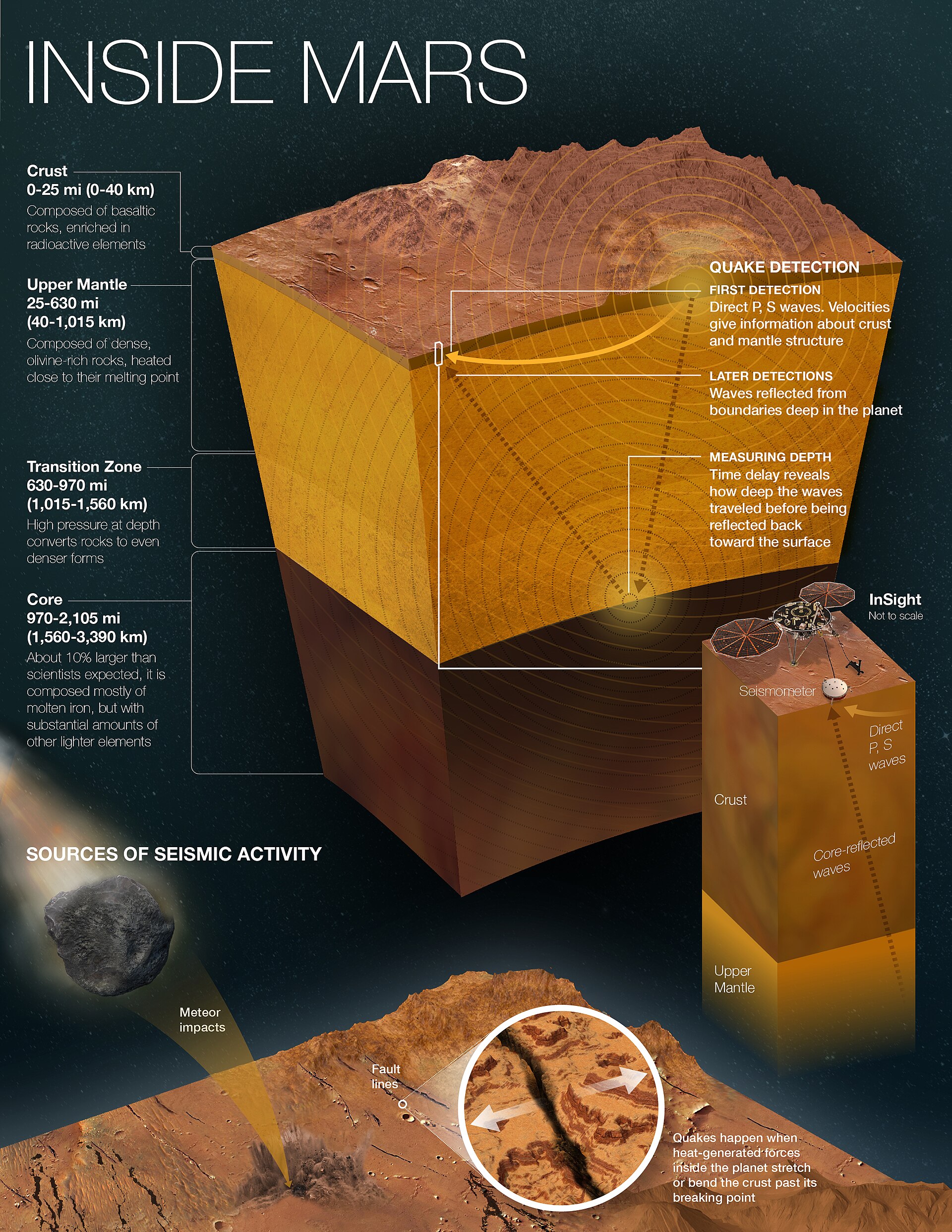
NASA infographic summarising the InSight-derived model of the — Fig. 56 interior of Mars. A vertical wedge through the planet shows a thin outer crust, a silicate mantle, and a large liquid iron-alloy core whose radius is now constrained by seismology. Annotations identify the seismometer SEIS on the surface and indicate ray paths of marsquakes and meteoroid impacts that travel through the planet to the single instrument. :width: 80%#

**Mars from a single seismometer.** NASA/JPL-Caltech infographic PIA25282 (public domain; 17 May 2022) summarising the interior model of Mars derived from the InSight mission’s SEIS instrument [Banerdt *et al.*, 2020]. With *one* broadband station on the surface, the inverse problem of §3–7 collapses to its hardest possible geometry: every “ray” begins at an unknown source location and ends at the same single receiver, and the resolution is governed entirely by the time–distance information available in surface reflections (PP, SS), core phases (PcP, ScS) and converted phases (SKS). **Reading exercise (geophysical reasoning):** with only one station, list which of the four resolution effects of Fig. 55 becomes the binding constraint on recovering Mars’s core radius, and explain in two sentences why adding meteoroid impacts as additional sources improves the inverse problem more than adding more marsquakes from the same source region would.

11. AI Literacy#

AI Literacy — Tool use and critical evaluation (LO-7)

Seismic tomography is increasingly AI-assisted, and this is where careful epistemic habits matter most. There are three places where machine learning currently sits inside a tomographic pipeline, each with its own failure modes.

1. ML phase picking (PhaseNet, EQTransformer). These models replace human picks with CNN predictions. Their failure modes are subtle: they sometimes miss emergent arrivals, they occasionally confound S on the vertical component with P, and their performance degrades in noise conditions unlike those in their training set (e.g., a picker trained on California data may perform worse in Cascadia). Good practice: always compare ML picks to a small set of manual picks on the same data before inverting.

2. ML-based tomographic solvers. Some recent work replaces the linear solver in Eq. (103) with a neural network that maps travel-time residuals directly to a 3-D model (e.g., Earle et al. 2023). These networks can hallucinate structure that is not in the data. Good practice: never trust an ML tomographic image that is not validated against a conventional least-squares inversion on the same data.

3. Language-model-based literature summarisation. A student might ask an AI assistant “what is the current best tomographic model of the Cascadia slab?” A plausible-sounding answer may cite invented papers and invented authors. Good practice: every citation an AI assistant produces should be verified directly — a paper whose DOI does not resolve, or whose title does not appear on the authors’ websites, is almost certainly fabricated.

Prompt to try. “Compare the Cascadia tomography models of Schmandt and Humphreys (2010) and Bodmer et al. (2018). What differences in slab geometry do they report, and why?” Then verify: do both papers exist? Does the model agree about the Juan de Fuca slab dip? If the assistant gives figures or numbers, are they traceable to specific tables or figure captions in the cited papers?

12. Concept Checks#

[LO-12.1] Write down the \(\mathbf{G}\) matrix for a \(3 \times 3\) grid of cells illuminated by three horizontal rays (top, middle, bottom) and three vertical rays (left, centre, right). Identify one model perturbation \(\delta\mathbf{m}\) that lies in the null space of \(\mathbf{G}\) — i.e., a perturbation that produces no change in any of the six travel times.
[LO-12.2] A tomographer damps an inversion with \(\varepsilon^2 = 0.01\) and recovers a slab with a \(V_P\) anomaly of \(+2\%\). They repeat the inversion with \(\varepsilon^2 = 0.1\) and the recovered amplitude drops to \(+1\%\). What does this tell you about the true amplitude of the anomaly? About the resolution of the image?
[LO-12.3] Looking at Figure Fig. 78, predict (i) where on the seafloor the subducted oceanic crust was created, and (ii) whether the mantle wedge partial-melt zone will appear as a positive or negative \(V_P\) anomaly, and by how many percent (order of magnitude).

13. Connections#

Previous lectures. Lecture 11 established the 1-D reference model PREM; this lecture perturbs it. The seismic phases you learned to identify in Lecture 11 are the data this lecture inverts.
Companion lab. Lab 6 guides students through (a) fetching teleseismic waveforms from IRIS for PNSN stations, (b) picking phase arrivals both manually and with PhaseNet, (c) comparing the pick residuals to AK135, and (d) mapping the residuals onto a simple 2-D tomographic image of the Cascadia slab.
Future lectures. Lectures 13-15 turn from subsurface imaging to active-source earthquake seismology — but the mathematical apparatus of this lecture (\(\mathbf{d} = \mathbf{G}\mathbf{m}\), damped least squares, null-space caution) reappears in earthquake location (Lecture 13) and moment-tensor inversion (Lecture 14). Learn it well now.


Course LOs addressed	LO-2, LO-3, LO-5, LO-7
Learning outcomes practiced	LO-OUT-B (compute travel-time residuals), LO-OUT-D (set up \(\mathbf{G}\mathbf{m}\) inversion), LO-OUT-E (interpret regularised model), LO-OUT-F (choose tomographic approach)
Prior lectures	Lecture 11 (PREM, global phases, 1-D Earth); Lecture 10 (forward/inverse framework, \(F\mathbf{m} = \mathbf{d}\))
Next lecture	Lecture 13 — Earthquake Phenomena I
Lab connection	Lab 3 extension: students invert a toy 2×2 slowness grid and explore how damping controls model roughness vs. data fit
Discussion connection	Discussion 6: Cascadia slab imaging — comparing seismic velocity anomalies to geological observations