Seismic Reflections II: Beyond the Flat-Layer Model

Seismic Reflections II: Beyond the Flat-Layer Model#

Prerequisites#

Students should be comfortable with Snell’s law (Lecture 5), acoustic impedance, the normal-incidence reflection coefficient \(R(0) = (Z_2-Z_1)/(Z_2+Z_1)\), and the flat-layer two-way travel-time hyperbola derived in Lecture 8.

1. From Ideal to Real: Five Assumptions That Fail#

In Lecture 8, the CMP stacking pipeline — sort, NMO correct, stack — produced a sharp zero-offset section from multi-offset data. That pipeline rested on five simplifying assumptions:

Reflectors are horizontal — the NMO hyperbola has no linear term in \(x\)
Only primary reflections reach the receiver — every event in the gather is a single-bounce wave
Reflecting interfaces are continuous — reflections come from planar surfaces, not isolated point scatterers
The recorded wavefield is noise-free — no ground roll, no air blast, no source-generated surface waves
Only travel times matter — amplitudes are constant with offset

None of these holds in a real survey. In the Cascadia accretionary wedge, fold-and-thrust structures produce reflectors dipping at 5–25°. Shallow water-bottom multiples dominate marine gathers. Fault-tip diffractions obscure thrust geometry. Ground roll overwhelms land data. And amplitude varies with incidence angle — carrying information about fluid content that travel times alone cannot provide.

This lecture relaxes each assumption in turn. For every complication, we follow the same progression:

Why it matters → What breaks → The math → How to fix it

2. Complication 1: Dipping Reflectors#

Assumption that fails: Reflectors are horizontal. In the Cascadia accretionary wedge, fold-and-thrust structures produce reflectors dipping at 5–25°, invalidating the symmetric NMO hyperbola from Lecture 8.

2.1 Why It Matters: The Geometry of Dip#

A reflector dipping at angle \(\delta\) from horizontal presents a different reflection geometry in the up-dip and down-dip directions from a common surface source. For down-dip shooting (receiver in the down-dip direction), each successive receiver is above a progressively deeper part of the reflector, and the two-way path increases faster than for a flat reflector at the same perpendicular depth \(h\). For up-dip shooting, the receiver looks toward the shallower part of the reflector, shortening the two-way path.

The result is an asymmetric travel-time curve: the same source–receiver configuration produces different arrival times depending on the survey direction.

2.2 What Breaks: CMP Reflection-Point Smear#

For a flat reflector, every trace in a CMP gather reflects from the same subsurface point — directly below the surface midpoint. For a dipping reflector, the reflection point migrates up-dip as offset increases (Fig. Fig. 30). A CMP gather over a dipping layer therefore samples a laterally smeared zone, not a single point. Standard NMO stacking produces a spatially blurred image in the presence of dip.

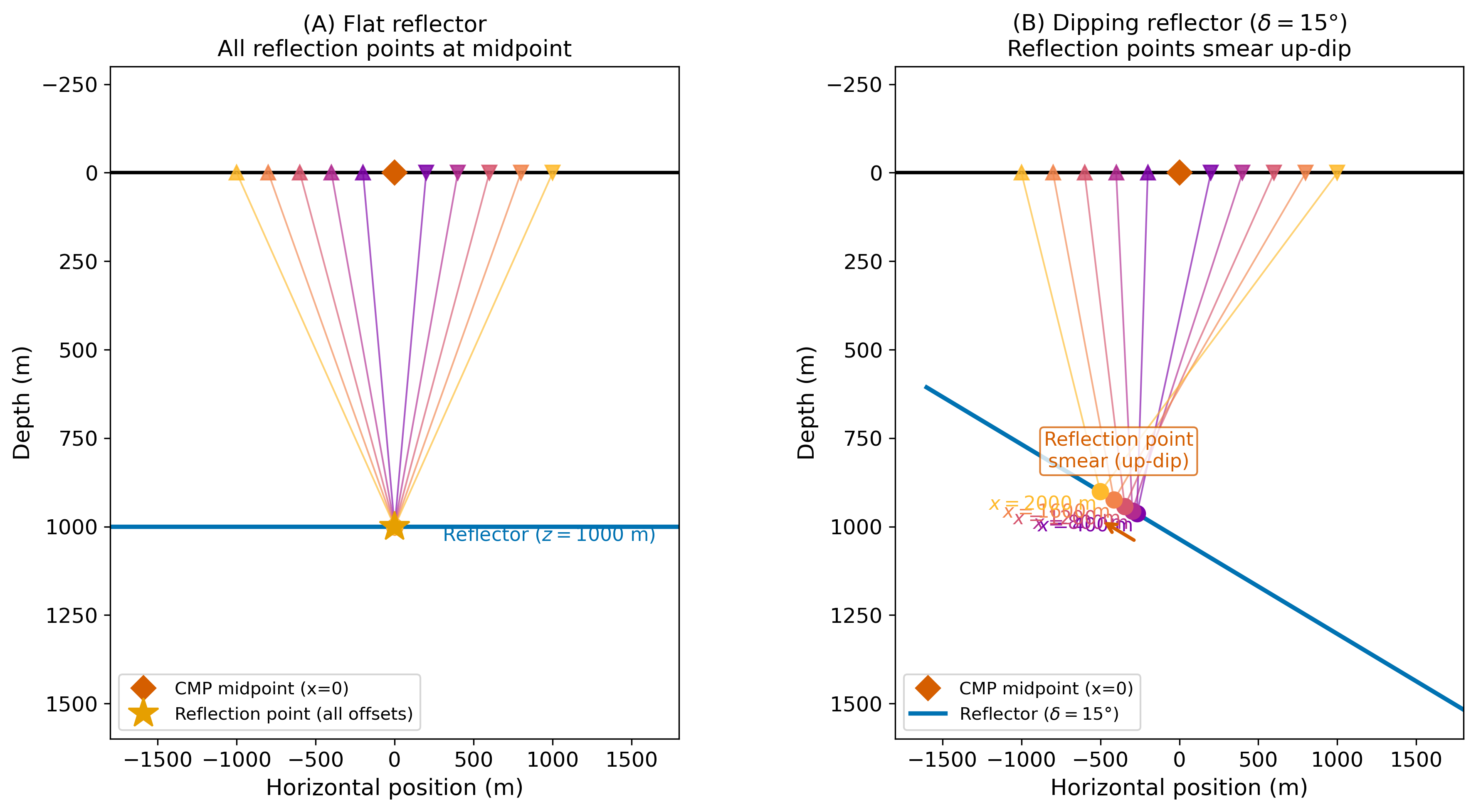
Two-panel figure. Left panel shows a flat horizontal reflector at 1000 m depth; all ray paths for different offsets in a CMP gather converge on the same single reflection point directly below the surface midpoint. Right panel shows a dipping reflector at 15 degrees; the reflection points are smeared up-dip at shallower depths as offset increases. — Fig. 30 **CMP reflection-point geometry for flat (left) and dipping (right) reflectors.** For a flat reflector, all traces in the CMP gather share the same reflection point. For a dipping reflector (\(\delta = 15°\)), the reflection point migrates up-dip with increasing offset. Stacking without a dip-moveout (DMO) correction averages over a spatially extended zone. [Python-generated: `assets/scripts/fig_cmp_dipping_scatter.py`]#

2.3 Exact Travel-Time Equation#

Using the image-point method, the exact two-way travel-time for a source at the origin and receiver at offset \(x\), with a reflector whose perpendicular distance from the source is \(h\) and dip angle \(\delta\), is

(78)#\[t_d(x) = \frac{1}{V_1}\sqrt{x^2 + 4h x\sin\delta + 4h^2} \quad \text{(down-dip)}\]

(79)#\[t_u(x) = \frac{1}{V_1}\sqrt{x^2 - 4h x\sin\delta + 4h^2} \quad \text{(up-dip)}\]

Both curves share the same zero-offset intercept \(t_0 = 2h/V_1\).

2.4 The Linear Term and Asymmetry#

Squaring and expanding:

(80)#\[t^2(x) = t_0^2 + \frac{x^2}{V_1^2} \pm \frac{2 t_0 \sin\delta}{V_1}\cdot x\]

The \(\pm(2 t_0 \sin\delta / V_1) \cdot x\) term — linear in \(x\) and absent in the flat-layer case — is the mathematical signature of dip. It produces:

Down-dip (+ sign): MORE moveout than flat → shallower apparent NMO velocity when fit with a flat-layer model
Up-dip (− sign): LESS moveout than flat → deeper apparent NMO velocity

The \(t^2\)–\(x^2\) relationship is therefore non-linear for dipping reflectors, making the linear regression incorrect.

Three-panel figure. Panel A shows geometry with source, up-dip and down-dip receivers, a green dipping reflector and ray paths. Panel B shows travel-time curves for flat (grey dashed), down-dip (orange), and up-dip (blue) shooting sharing the same t0. Panel C shows the t-squared x-squared relationship with curved non-linear trends for the dipping cases and a green dotted tangent showing V_NMO = V1/cos-delta. 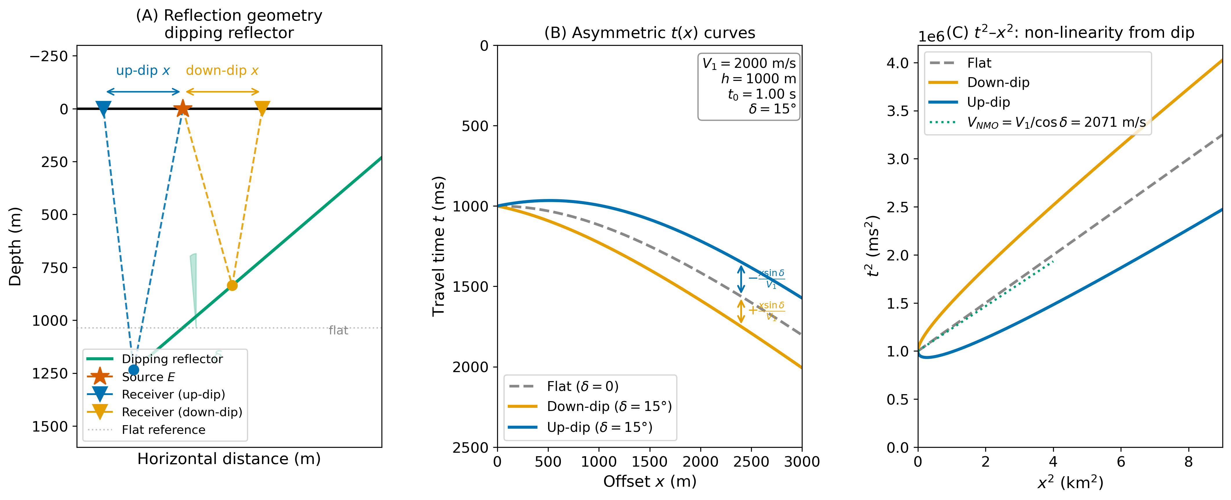— Fig. 31 **Dipping-layer travel-time asymmetry.** (A) Geometry. (B) \(t(x)\) curves: down-dip arrivals are delayed relative to the flat-layer case; up-dip arrivals are early. (C) \(t^2\)–\(x^2\) plot: non-linear trends for dipping cases contrast with the straight flat-layer line. The green dotted tangent has slope \(1/V_\mathrm{NMO}^2 = \cos^2\delta/V_1^2\). [Python-generated: `assets/scripts/fig_dipping_layer_geometry.py`]#

2.5 What Breaks: NMO Velocity for Dipping Layers#

Taylor-expanding \(t_d(x)\) around \(x = 0\), the quadratic coefficient gives:

(81)#\[V_\mathrm{NMO,dip} = \frac{V_1}{\cos\delta}\]

This is larger than \(V_1\); fitting a flat-layer NMO model to data over a dipping reflector overestimates the subsurface velocity.

2.6 The Fix: Recovering True Velocity and Dip#

From two surveys — one down-dip and one up-dip — the true velocity and dip angle can be recovered:

(82)#\[V_1 = \frac{2\,V_d\,V_u}{V_d + V_u}, \qquad \sin\delta = \frac{V_u - V_d}{V_u + V_d}\]

In practice, dip-moveout (DMO) correction is applied after NMO correction to reposition the reflection points to a common location before stacking.

With dip accounted for, the next complication is unwanted energy from waves that bounce more than once.

3. Complication 2: Multiple Reflections#

Assumption that fails: Only primary reflections reach the receiver. In reality, seismic energy bounces multiple times between the free surface and subsurface reflectors, generating coherent events that mimic primaries.

A multiple is a seismic event that has undergone more than one reflection before reaching the receiver. Multiples are coherent and appear as hyperbolic events in the CMP gather; they are a primary source of false structure in seismic sections.

3.1 Types of Multiples#

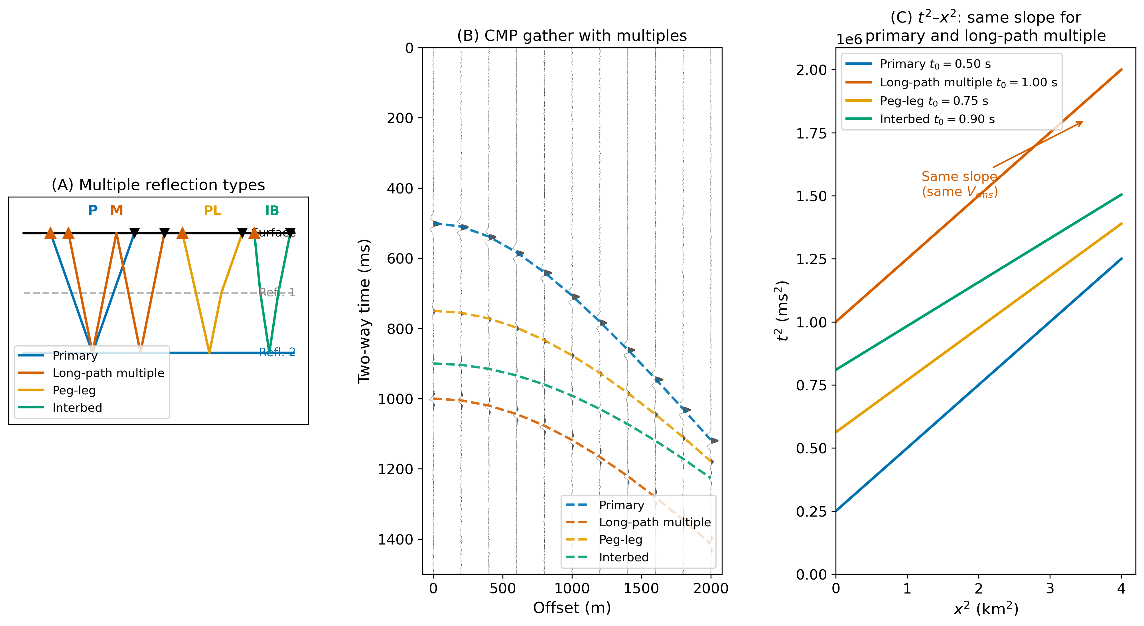
Three-panel figure. Panel A shows ray-path diagrams for four multiple types: primary P, long-path multiple M, peg-leg PL, and interbed IB. Panel B shows the synthetic CMP gather with four hyperbolic events. Panel C shows the t-squared x-squared plot where the long-path multiple and primary have the same slope (same V_rms) but the multiple has double the intercept. — Fig. 32 **Multiple reflection types.** (A) Ray paths: primary (P), long-path surface multiple (M), peg-leg (PL), and interbed (IB). (B) Synthetic CMP gather. (C) \(t^2\)–\(x^2\) plot: the long-path multiple and its parent primary have **identical slopes** (same \(V_\mathrm{rms}\)) — this is the central challenge for NMO stacking. [Python-generated: `assets/scripts/fig_multiple_types.py`]#

The long-path (surface) multiple travel-time is:

(83)#\[t_\mathrm{mult}^2(x) = (2\,t_0)^2 + \frac{x^2}{V_\mathrm{rms}^2}\]

This has the same NMO velocity as the primary but double the zero-offset TWTT. Because NMO correction simultaneously flattens both, stacking will not suppress the multiple.

3.2 The Fix: Multiple Suppression#

Modern workflows use surface-related multiple elimination (SRME): the observed wavefield is autocorrelated with itself to predict the multiple waveforms, which are then adaptively subtracted. Deep-learning approaches train encoder-decoder networks to separate primaries from multiples in the \(\tau\)-\(p\) domain.

With multiples suppressed, we turn to energy scattered by point-like discontinuities rather than planar interfaces.

4. Complication 3: Diffractions#

Assumption that fails: Reflecting interfaces are continuous surfaces. At sharp discontinuities — fault tips, unconformity edges, channel boundaries — the wavefront scatters in all directions.

4.1 Huygens Principle and Point Scatterers#

Every point on a wavefront acts as a secondary source of spherical wavelets (Huygens’s principle). At a sharp subsurface discontinuity — a fault tip, an unconformity edge, a channel boundary — the incident wave excites new secondary spherical waves. These diffractions carry energy in all directions equally.

For a point scatterer at \((x_s, z_s)\) in a medium of velocity \(V_1\), the diffraction travel time is:

(84)#\[t_\mathrm{diff}(x) = \frac{2}{V_1}\sqrt{(x - x_s)^2 + z_s^2}\]

This is a hyperbola with vertex at \((x_s,\, 2z_s/V_1)\).

Three-panel figure. Panel A shows a depth cross-section with a flat blue-dashed reflector at 600 m and a fault-tip scatterer at 1000 m with orange ray paths fanning to surface receivers. Panel B shows the t(x) curves for the flat-reflector primary (blue dashed) and fault-tip diffraction (red solid). Panel C shows the synthetic zero-offset section with the flat primary and diffraction hyperbola visible. 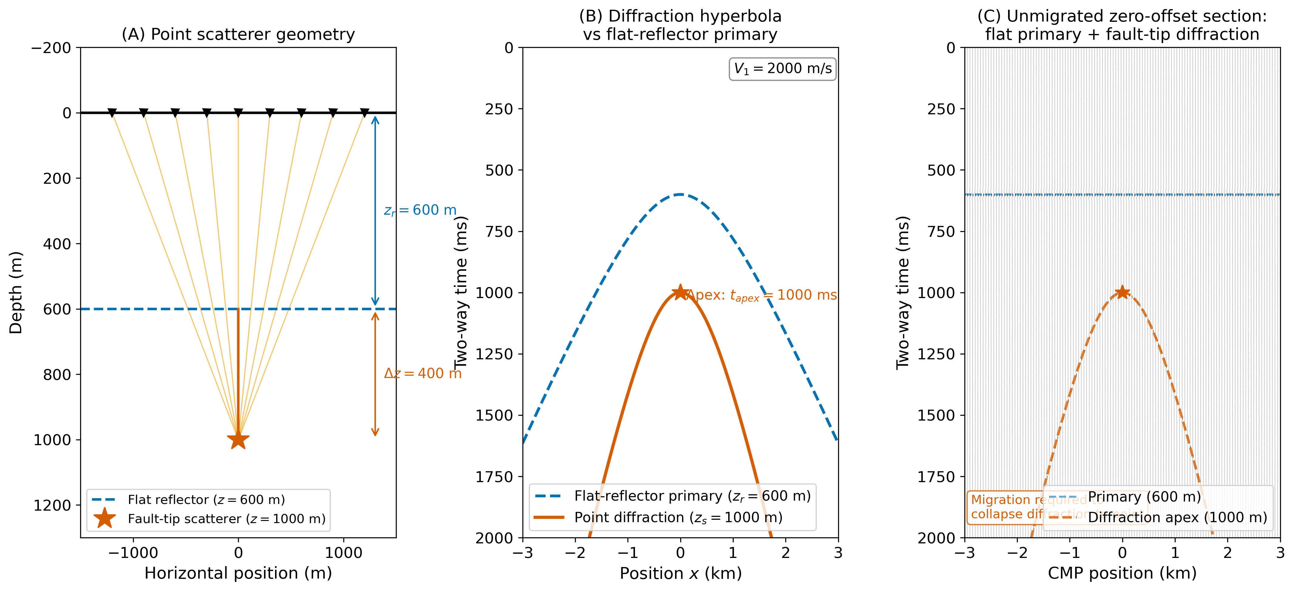— Fig. 33 **Point diffraction from a fault-tip scatterer.** (A) Subsurface model. (B) Travel-time curves: the diffraction hyperbola extends uniformly across the entire receiver array. (C) Synthetic zero-offset section. Migration collapses the hyperbola to the fault-tip point, recovering the true geometry. [Python-generated: `assets/scripts/fig_diffraction_hyperbola.py`]#

4.2 The Fix: Migration#

An unmigrated seismic section displays the hyperbolic diffraction rather than the point; fault terminations appear as fan-shaped energy patches. A syncline bounded by two dipping reflectors produces a “bowtie” pattern. Seismic migration — the topic of Lecture 10 — collapses diffractions and repositions dipping events to their true subsurface locations.

Diffractions will be collapsed by migration (Lecture 10). Meanwhile, another class of unwanted energy — coherent noise from surface waves — must be removed before stacking.

5. Complication 4: Coherent Noise and Signal Enhancement#

Assumption that fails: The recorded wavefield contains only reflected body waves. A raw shot gather is dominated by surface waves (ground roll), direct arrivals, and other coherent noise that masks the reflections we seek.

5.1 Coherent Noise Types#

A raw shot gather contains several coherent noise types alongside desired reflections:

Direct wave (\(V \approx V_1\)): linear first arrival, easily muted
Ground roll (Rayleigh wave; \(V \approx 200\)–500 m/s): high amplitude, low frequency (5–20 Hz), dispersive; dominates land gathers at short and medium offsets
Air blast (\(V \approx 340\) m/s): muted by velocity filter
Head wave (\(V > V_1\)): muted before NMO correction

5.2 The Fix: f–k Velocity Filtering#

In the frequency-wavenumber (\(f\)–\(k\)) domain, events with apparent velocity \(V_\mathrm{app}\) map to the line \(k = f/V_\mathrm{app}\). Ground roll occupies the high-\(|k|\) fan region. A velocity filter rejects all \(|k| > f/V_\mathrm{cutoff}\):

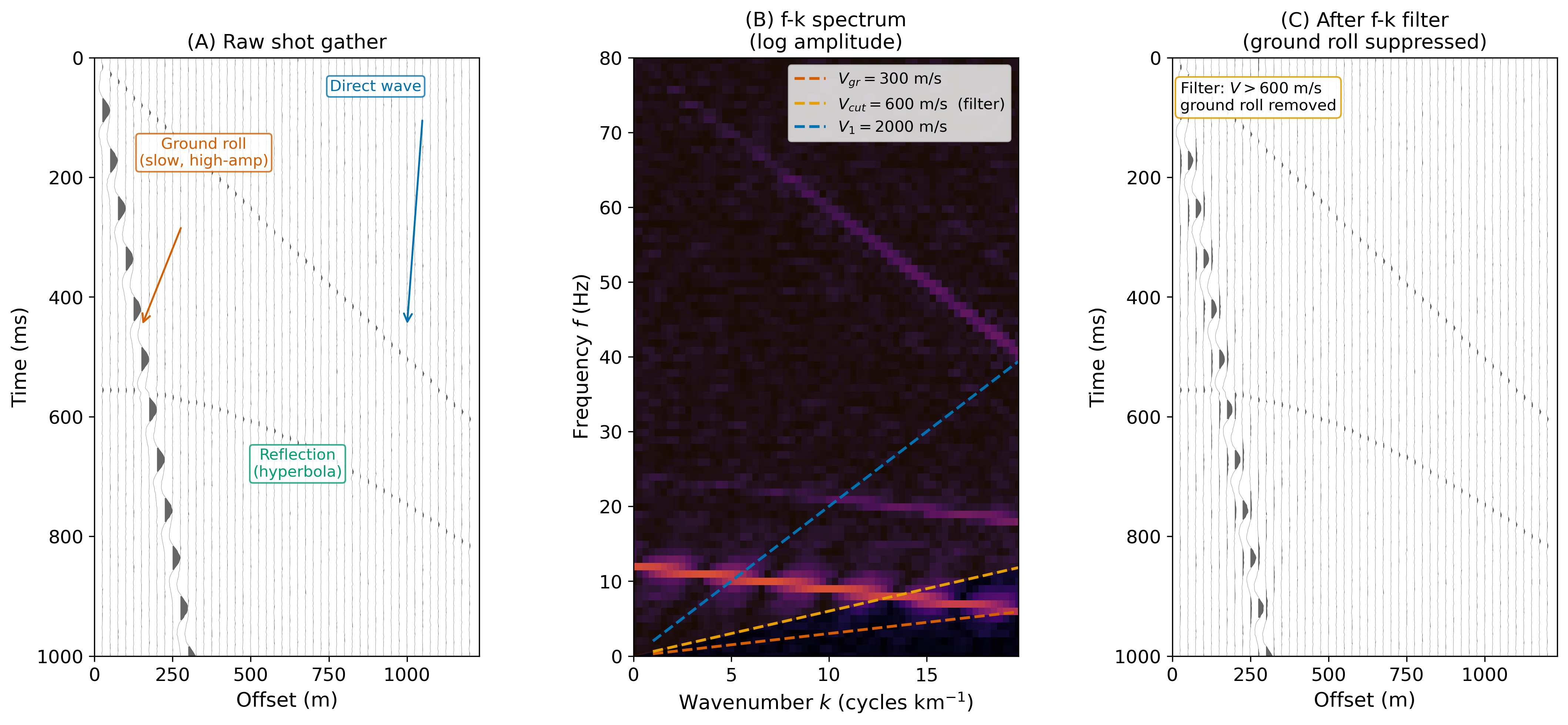
(85)#\[\begin{split}\mathcal{M}(f, k) = \begin{cases} 1 & |k| < f / V_\mathrm{cutoff} \\ 0 & \text{otherwise} \end{cases}\end{split}\]

Three-panel figure. Panel A shows a raw shot gather with labelled ground roll, direct wave, and hyperbolic reflection. Panel B shows the f-k amplitude spectrum with velocity fan lines at 300, 600, and 2000 m/s. Panel C shows the filtered gather with ground roll removed and the reflection hyperbola now clearly visible. — Fig. 34 **Ground-roll suppression by f–k velocity filtering.** (A) Raw gather: ground roll dominates at small offsets. (B) f–k spectrum: the slow fan of ground roll is separated from fast reflection events; filter mask at \(V_\mathrm{cutoff} = 600\) m/s shown in orange. (C) Filtered gather: ground roll attenuated, reflection hyperbola visible. [Python-generated: `assets/scripts/fig_ground_roll_fk.py`]#

5.3 Stacking Fold and SNR#

After NMO correction and noise filtering, the stacked trace SNR improves as:

(86)#\[\mathrm{SNR}_\mathrm{stack} = \sqrt{N_\mathrm{fold}} \times \mathrm{SNR}_\mathrm{single}\]

A 48-fold survey improves SNR by a factor of \(\approx 7\). Modern dense 3D surveys achieve fold \(> 200\).

With noise suppressed and travel times corrected, we can finally examine what the amplitudes themselves reveal about subsurface rock and fluid properties.

6. Complication 5: Amplitude Versus Offset#

Assumption that fails: Only travel times carry useful information. In fact, how the reflection amplitude changes with incidence angle reveals the fluid content of subsurface rocks — information invisible to NMO velocity analysis alone.

6.1 Oblique-Incidence Reflectivity#

For a plane P-wave incident at angle \(\theta_i\) on a planar interface, the reflected and transmitted amplitudes are governed by the Zoeppritz equations. For moderate angles (\(\theta_i < 30°\)), the Shuey (1985) two-term approximation gives:

(87)#\[R(\theta_i) \approx R(0) + G\,\sin^2\theta_i\]

where \(R(0) = (Z_2 - Z_1)/(Z_2 + Z_1)\) is the normal-incidence reflection coefficient (intercept) and \(G\) is the AVO gradient, sensitive to the contrast in \(V_P/V_S\) ratio across the interface. Gas substitution strongly lowers \(V_P\) while leaving \(V_S\) nearly unchanged, producing a large distinctive change in \(G\).

6.2 AVO Classes#

Two-panel figure. Panel A shows reflection coefficient R versus incidence angle for AVO Classes I through IV and IIp. Class I starts positive and decreases. Class II starts near zero with polarity reversal. Class III starts negative and brightens with offset (gas sand). Class IV starts negative and dims. Panel B shows the AVO crossplot of intercept R(0) versus gradient G with scatter clusters for each class and background trend line. 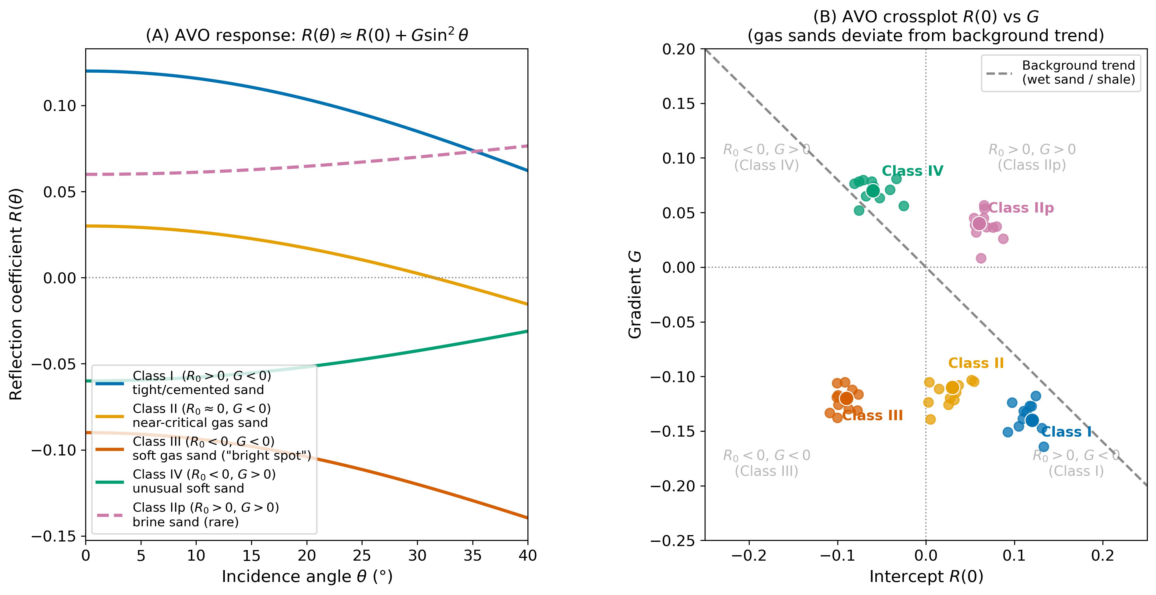— Fig. 35 **AVO classes and the \(R(0)\)–\(G\) crossplot.** (A) \(R(\theta)\) curves: Class III gas sands brighten with offset (\(R(0) < 0\), \(G < 0\)); Class I tight sands dim. (B) Crossplot: wet sands and shales cluster along the background trend; gas sands deviate toward the lower left. [Python-generated: `assets/scripts/fig_avo_classes.py`]#

Class I (\(R(0) > 0\), \(G < 0\)): Hard sand or cemented rock; amplitude decreases with offset.
Class II (\(R(0) \approx 0\), \(G < 0\)): Near-zero normal-incidence contrast; polarity reversal at intermediate angle.
Class III (\(R(0) < 0\), \(G < 0\)): Soft gas sand; amplitude increases with offset — the classical bright spot direct hydrocarbon indicator (DHI).
Class IV (\(R(0) < 0\), \(G > 0\)): Amplitude decreases with offset despite a negative intercept; overpressured or very shallow gas sands.

6.3 The AVO Crossplot and Fluid Discrimination#

Plotting \(R(0)\) against \(G\) for all reflection events in a 3D survey produces the AVO crossplot. Background wet sands and shales cluster along a “fluid line” (\(G \approx -R(0)\)). Gas-saturated sands deviate toward more negative \(G\) values (Classes II, III). The deviation from the background trend is the primary diagnostic for fluid content beyond what impedance alone resolves.

7. Worked Example: Dipping-Layer Survey#

Given: A 2D survey over a thrust-fault reflector. Perpendicular depth \(h = 800\) m, \(V_1 = 2000\) m/s, \(\delta = 10°\).

Quantity	Formula	Result
Zero-offset TWTT	\(t_0 = 2h/V_1\)	0.80 s
NMO velocity (dipping)	\(V_\mathrm{NMO} = V_1/\cos\delta\)	2031 m/s
Down-dip at \(x = 2400\) m	Eq. (78)	1.553 s
Up-dip at \(x = 2400\) m	Eq. (79)	1.322 s

Check apparent velocities: \(V_d \approx 1704\) m/s, \(V_u \approx 2421\) m/s → \(\sin\delta = (2421-1704)/(2421+1704) = 0.174 \approx \sin10°\) ✓

Concept Check

A CMP gather over a 12° dipping reflector is NMO-corrected using the flat-layer formula \(V_\mathrm{NMO} = V_1\). Will the corrected reflectors be over- or under-corrected? Explain using Eq. (81).
A long-path multiple arrives at \(t = 1.4\) s at zero offset with \(V_\mathrm{rms} = 2400\) m/s. At what zero-offset time does its parent primary arrive? Compute the depth to the reflecting horizon.
A seismic section shows a hyperbolic event that broadens uniformly across all offsets without attenuating. Is this a primary reflection or a diffraction? What must be done to recover the true geological feature?

8. SOTA: Deep Learning in Reflection Seismic Processing#

8.1 Supervised Denoising with U-Nets#

The dominant deep-learning architecture for seismic denoising is the U-Net — a fully convolutional encoder-decoder network trained to map a noisy seismic gather to a denoised output:

\[\hat{\mathbf{d}}_\mathrm{clean} = f_\theta(\mathbf{d}_\mathrm{noisy}), \qquad \theta^* = \arg\min_\theta \|\mathbf{d}_\mathrm{clean}^\mathrm{train} - f_\theta(\mathbf{d}_\mathrm{noisy}^\mathrm{train})\|^2\]

Skip connections between the encoder and decoder layers preserve fine spatial detail that would otherwise be lost in the downsampling path.

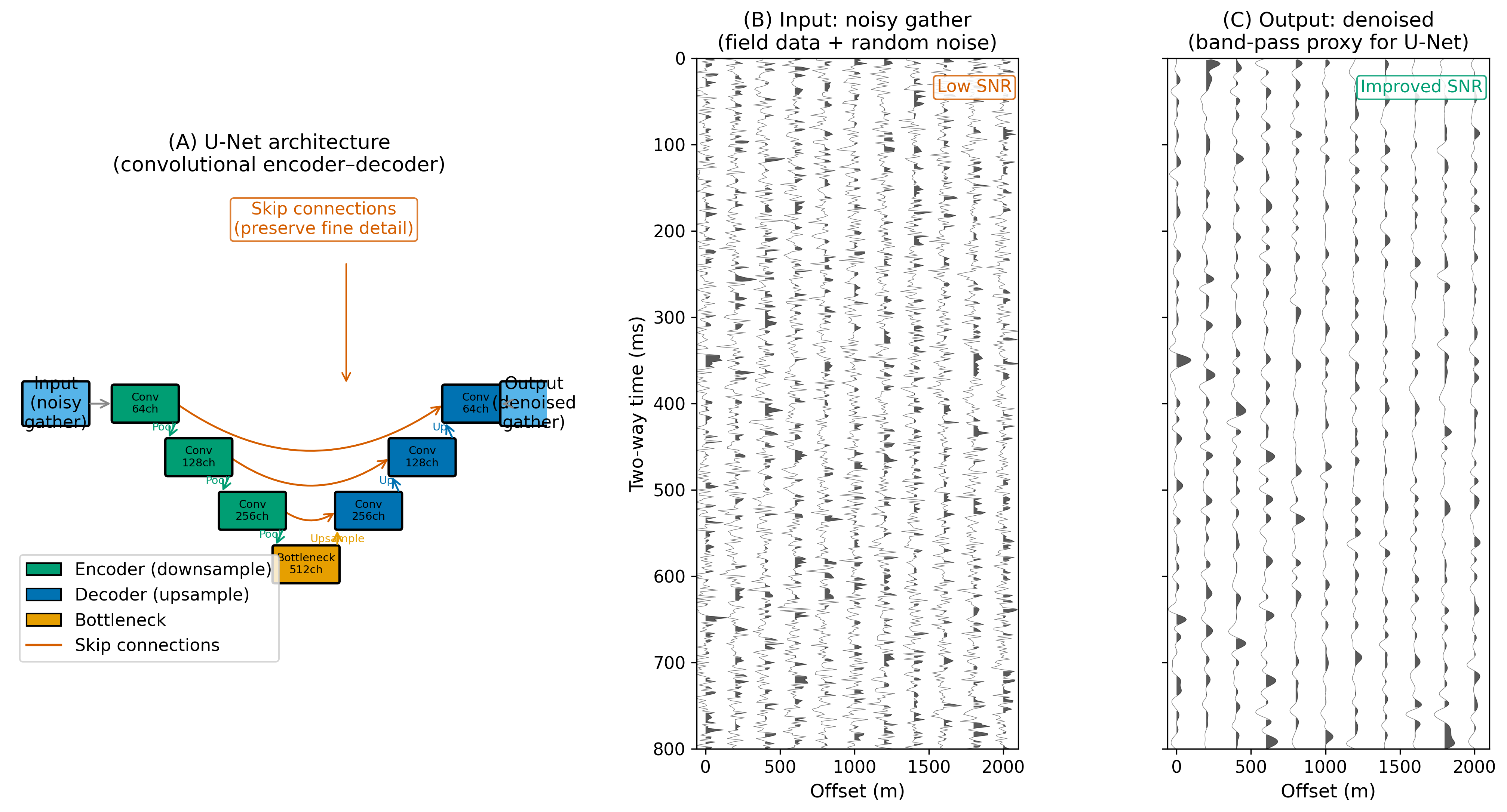
Three-panel figure. Panel A shows a U-Net architecture schematic with encoder (green boxes), bottleneck (orange box), decoder (blue boxes), and red skip connections. Panel B shows a noisy synthetic CMP gather. Panel C shows the denoised output with improved SNR. — Fig. 36 **U-Net architecture for seismic denoising.** (A) Encoder-decoder with skip connections. (B) Noisy input gather. (C) Denoised output. A real U-Net learns the noise distribution from training data; band-pass filtering is shown here as a proxy. [Python-generated: `assets/scripts/fig_dl_denoising_concept.py`]#

8.2 Self-Supervised and Foundation Models#

A limitation of supervised U-Nets is the need for paired clean/noisy training data, which is unavailable for real field datasets. Self-supervised methods train entirely on the observed noisy data by exploiting the statistical property that noise is spatially uncorrelated while signal is coherent.

Seismic foundation models (e.g. SeisFoundation, SegFM) are large pretrained vision transformers fine-tuned on seismic images that can perform multiple tasks — denoising, horizon picking, facies classification — from a single model backbone.

8.3 Open Challenges#

Domain shift: networks trained on synthetic gathers frequently fail on field data because real noise is non-stationary and geologically correlated.
Physics inconsistency: a denoised gather may violate reciprocity, polarity conventions, or AVO relationships physically present in the original data.
Interpretability: it is difficult to determine whether an amplitude anomaly in a DL-denoised section is a true DHI or a network artifact.

9. Course Connections#

The dipping-layer travel-time equation (§2) is the direct extension of the flat-layer hyperbola (\(\delta \to 0\) recovers the standard reflection hyperbola). The additional linear term motivates DMO correction, which is a special case of the migration operator discussed in Lecture 10.

Diffraction hyperbolae (§4) are the building block of Kirchhoff migration (Lecture 10, §3): migration collapses diffractions by summing amplitudes along the diffraction curve.

The AVO gradient \(G\) involves \(V_P/V_S\), which connects to density constraints available from the gravity module (Lectures 18–22): density is related to both impedance (\(Z = \rho V_P\)) and AVO (\(G\) depends on \(\Delta\rho/\rho\)).

10. Research Horizon#

Current Research Highlights (2022–2025)

Learned multiple suppression uses deep learning in the \(\tau\)-\(p\) domain to achieve adaptive subtraction without the wave-equation modelling required by SRME, reducing computational cost by 1–2 orders of magnitude (Xiong et al. 2023).

Sparse-shot acquisition and DL interpolation trains networks to reconstruct densely sampled shot gathers from sparse acquisitions, enabling 4D time-lapse surveys at a fraction of traditional acquisition cost (Mosher et al. 2023).

Physics-informed AVO inversion embeds Zoeppritz boundary conditions as hard constraints in a neural-network inversion, ensuring that recovered \(V_P/V_S\) profiles satisfy the governing physics rather than merely fitting observed amplitudes (Zhang et al. 2024).

For students interested in graduate research: EarthScope SSBW workshops and the SCOPED project (scoped.codes) are entry points. The IRIS/EarthScope AVO module provides open datasets.

11. Societal Relevance#

Why It Matters Beyond the Classroom

Direct Hydrocarbon Indicators: The AVO Class III “bright spot” is the most widely used DHI in exploration. False positive identifications — attributing a bright reflection to gas when it is caused by a shallow coal seam, a hard carbonate layer, or a DL denoising artifact — have led to costly dry wells. The \(R(0)\)–\(G\) crossplot uncertainties directly inform decisions worth hundreds of millions of dollars.

Carbon Capture and Storage (CCS): AVO analysis is now central to characterizing CO₂ storage reservoirs and monitoring injection plumes — where accurate fluid discrimination directly affects the long-term security of millions of tonnes of stored CO₂.

Cascadia: The updip extent of the décollement’s seismic coupling is constrained by the impedance contrast between unconsolidated accretionary sediment and the overriding plate. Whether a bright spot at the plate interface is a fluid-saturated zone (Class III AVO) or a cemented carbonate zone (Class I) affects estimates of seismic moment release and future Cascadia rupture magnitude.

For further exploration: IRIS/EarthScope AVO educational module (CC-BY, iris.edu/hq/inclass/lesson/avo); Shuey (1985) is freely accessible and remains the canonical reference.

AI Literacy — Epistemics: Interrogating a Seismic Interpretation#

AI Prompt Lab

Ask an AI assistant to interpret: “A bright, negative-polarity reflection at 1.8 s TWTT with amplitude that increases strongly with offset on a marine gather acquired over a Paleogene sandstone reservoir.”

Before accepting the response, apply the epistemics framework:

What evidence distinguishes this from a multiple? (If it were a long-path multiple, what would its parent primary TWTT be? Does a primary exist at 0.9 s on the section?)
What evidence distinguishes it from a hard kick at the base of a fast layer? (Negative polarity can also come from impedance decreasing from dense limestone into soft shale.)
What data would confirm the gas interpretation? (Well control, fluid substitution modelling, 4D time-lapse survey, CSEM/MT resistivity data.)

Document: (a) what the AI identified correctly; (b) what the AI failed to flag as an alternative explanation; (c) what additional data the AI suggested or failed to suggest.


Course LOs addressed	LO-1 (multiples, diffractions, AVO physics), LO-2 (dipping-layer t-x math, Shuey coefficients), LO-3 (DMO concept, velocity analysis for dipping layers), LO-4 (flat-layer assumptions and when they break), LO-5 (figure generation in Lab 3), LO-7 (AI/ML tools evaluated critically)
Learning outcomes	LO-OUT-A through D, G, H
Prior lecture	Lecture 8 — Introduction to Seismic Reflection (flat-layer travel time, NMO, CMP stacking, velocity analysis)
Next lecture	Lecture 10 — Migration & Velocity–Image Duality
Lab connection	Lab 3 Part 6 (dipping-layer CMP gather; measure up-dip/down-dip velocities; apply f-k filter)