Seismic Reflections I: Flat-Layer Travel Time, NMO, and CMP Stacking

Seismic Reflections I: Flat-Layer Travel Time, NMO, and CMP Stacking#

Prerequisites#

Students should be comfortable with acoustic impedance (\(Z = \rho V\)), Snell’s law at oblique incidence (Lecture 5), the concept of the CMP gather, and basic signal processing (Fourier transform, SNR definition). The refraction travel-time equation (Lectures 6–7) provides the contrasting context.

1. The Geoscientific Question#

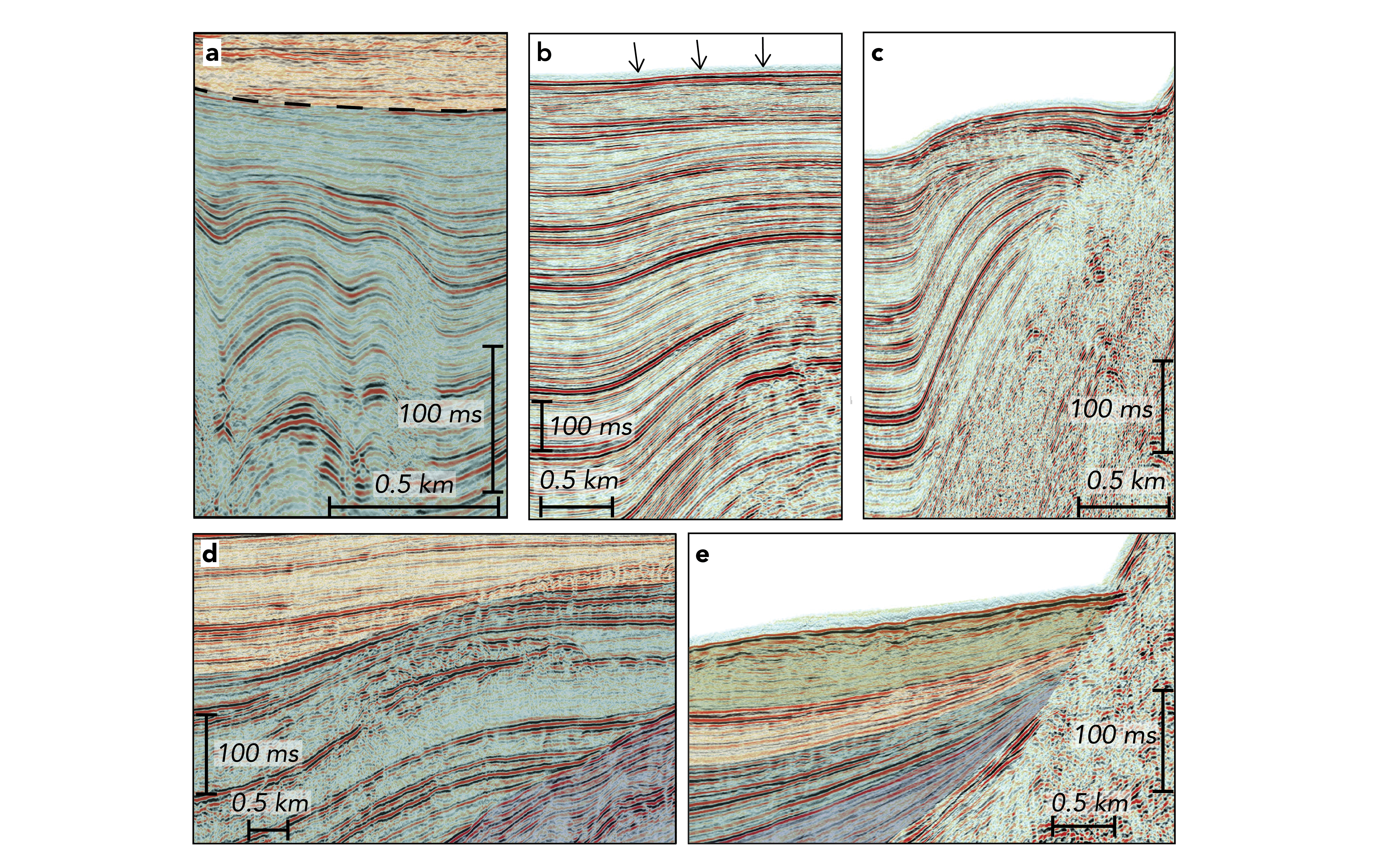
Five annotated sparker multi-channel seismic reflection panels (a–e) from the Cascadia accretionary wedge, offshore Washington, showing typical stratigraphic and deformational patterns. — Fig. 29 Fig. 2 from Ledeczi *et al.* [2024], *Seismica* 2(4). Licensed CC BY 4.0. Reproduced unmodified. Panels show (a) inactive fold with postdeformational strata, (b) active fault-propagation fold, (c) active fold with seafloor signature, (d) onlapping seismic facies, (e) stratal thinning indicating recent tectonic activity.#

Begin by looking at Fig. 29: a real seismic reflection section from the Cascadia accretionary wedge offshore Washington. The horizontal axis is distance along the survey line; the vertical axis is two-way travel time (TWTT) — not depth. Bright bands mark interfaces with large impedance contrast; dark zones correspond to gradational or low-contrast boundaries. The lateral variation in reflector character reveals folds, faults, and basin-fill history.

This image is the product of seismic reflection processing. This lecture develops the physics and methodology that build it, starting from a single reflected pulse and working up to the full stacked cross-section.

In contrast to refraction methods, which require the refracted wave to return along the surface and can only constrain velocity in the shallowest layers, reflection surveys image structure at any depth — from the shallow sedimentary column to the Moho and beyond.

2. Reflection Physics#

2.1 Acoustic Impedance#

The acoustic impedance of a layer is the product of density \(\rho\) and P-wave velocity \(V_P\):

(67)#\[Z = \rho\, V_P \quad [\text{Pa·s/m} = \text{kg m}^{-2}\text{s}^{-1}]\]

Impedance contrasts cause reflections. A high-impedance layer (dense, fast rock) strongly reflects downgoing energy.

2.2 Normal-Incidence Reflection and Transmission#

At normal incidence (\(\theta = 0\)), the reflection coefficient \(R\) and transmission coefficient \(T\) follow directly from boundary conditions (continuity of acoustic pressure and particle velocity):

(68)#\[R = \frac{Z_2 - Z_1}{Z_2 + Z_1}, \qquad T = \frac{2 Z_2}{Z_1 + Z_2}\]

Note: \(|R| \leq 1\) and the relationship \(R + T \cdot (Z_1/Z_2) = 1\) conserves energy. Typical crustal interfaces have \(|R| = 0.01\)–\(0.15\); the water–seafloor interface \(|R| \approx 0.25\).

2.3 Energy Reflection and Transmission Coefficients#

The fraction of energy (intensity) reflected and transmitted:

(69)#\[\mathcal{R} = R^2, \qquad \mathcal{T} = 1 - R^2 = \frac{4 Z_1 Z_2}{(Z_1 + Z_2)^2}\]

For a typical sedimentary contrast (\(R = 0.10\)), only 1% of energy is reflected and 99% is transmitted — which is why reflections are weak and stacking is essential.

2.4 The Reflectivity Profile#

A synthetic seismogram for a 1D layered Earth convolves the reflectivity series \(r(t) = \{R_1, R_2, \ldots\}\) with the source wavelet \(w(t)\):

\[d(t) = w(t) * r(t) = \sum_i R_i\, w(t - t_{0,i})\]

where \(t_{0,i} = 2 z_i / V_i\) is the two-way travel time to reflector \(i\). This convolutional model is the foundation of seismic interpretation: picking a reflector on a seismic section reads the acoustic impedance structure of the crust.

3. The Signal-to-Noise Problem#

The fundamental challenge of reflection seismology is that reflections are weak. Typical sedimentary interfaces have \(|R| = 0.01\)–\(0.15\), meaning only 1–2% of seismic energy reflects at any one boundary. Reflected P-waves are 1–3 orders of magnitude weaker than the direct first arrival, and the same receiver array simultaneously records surface waves, head waves, and scattered energy.

A single source–receiver trace is almost never enough to detect a reflector above ambient noise.

3.1 Stacking as the Solution#

Record the same reflection from \(N_\mathrm{fold}\) different source–receiver offsets. Because the reflection signal is coherent across traces (it arrives at a predictable time governed by geometry) while noise is incoherent:

Signal adds proportionally to \(N_\mathrm{fold}\)
Noise adds proportionally to \(\sqrt{N_\mathrm{fold}}\)

After normalising:

\[\mathrm{SNR}_\mathrm{stack} = \sqrt{N_\mathrm{fold}} \times \mathrm{SNR}_\mathrm{single}\]

For a 96-fold survey: \(\sqrt{96} \approx 10\times\) SNR improvement. This is the primary motivation for the Common Midpoint (CMP) method.

3.2 The Alignment Problem#

“Stacking” only works if the reflection signal on each trace is aligned to the same arrival time. But traces at different offsets record the reflector at different travel times — the arrival traces out a hyperbola in the offset–time plane. We must first understand this hyperbola (§4), correct for it (§5), and only then can we meaningfully stack (§9).

4. Travel Time for a Flat Horizontal Reflector#

4.1 The Image-Point Construction#

For a flat reflector at depth \(h\) with velocity \(V_1\) above it, the travel time from source at origin to surface receiver at offset \(x\) (down-path + up-path) can be computed using the method of images: reflect the source through the interface to create an image source at \((0, -h)\). The total raypath length is the straight-line distance from the image source to the receiver:

\[\ell(x) = \sqrt{x^2 + (2h)^2}\]

4.2 The Reflection Hyperbola#

Dividing by \(V_1\):

(70)#\[t(x) = \frac{\sqrt{x^2 + 4h^2}}{V_1}\]

Squaring:

(71)#\[t^2(x) = t_0^2 + \frac{x^2}{V_1^2}\]

where \(t_0 = 2h/V_1\) is the zero-offset two-way travel time. This is the equation of a hyperbola in the \(t\)–\(x\) plane, with:

Asymptotic slope \(\pm 1/V_1\) (straight lines at large \(x\))
Vertex at \((0, t_0)\)
Curvature controlled by \(h/V_1\): deep reflectors are flatter hyperbolas

Key insight

Plotting \(t^2\) vs \(x^2\) transforms the reflection hyperbola into a straight line with slope \(1/V_1^2\) and intercept \(t_0^2\). This is the foundation of velocity analysis: a linear regression on \(t^2\)–\(x^2\) simultaneously recovers \(h = V_1 t_0 / 2\) and \(V_1\).

5. Normal Moveout (NMO) Correction#

5.1 Definition#

The normal moveout is the incremental travel-time delay at offset \(x\) relative to zero offset:

(72)#\[\Delta t_\mathrm{NMO}(x) = t(x) - t_0 = \sqrt{t_0^2 + \frac{x^2}{V_\mathrm{NMO}^2}} - t_0\]

For small-to-moderate offsets (\(x \ll V_\mathrm{NMO} t_0\), i.e. \(x < h\)), the Taylor expansion gives:

(73)#\[\Delta t_\mathrm{NMO}(x) \approx \frac{x^2}{2\, V_\mathrm{NMO}^2\, t_0}\]

5.2 Applying NMO#

The NMO correction shifts each trace in the CMP gather upward by \(\Delta t_\mathrm{NMO}(x)\). After a correct NMO correction (using the true velocity \(V_1\)), all traces in the gather show the reflection at the same time \(t_0\). The gather is then said to be flattened — which is exactly the alignment step that makes the stacking argument from §3 work.

5.3 NMO Stretch#

At large offsets, the NMO correction is asymptotically large; the corrected wavelet is stretched in time (“NMO stretch”). Stretched traces at offsets \(x > x_\mathrm{mute}\) are discarded before stacking. The mute zone typically excludes \(x/h > 1.0\)–\(1.5\).

6. Acquisition Geometry and the CMP Gather#

With the hyperbola and NMO framework in hand, we can now understand how the data are collected to make stacking possible.

6.1 Shot Gather and CMP Gather#

A shot gather collects all receiver traces from a single source. Sources and receivers are arranged in a 2D line (or 3D grid), typically spaced \(\Delta x = 12.5\)–\(25\) m. The source–receiver offset \(x\) ranges from near-trace (\(x \approx \Delta x\)) to far-trace (\(x \approx N\Delta x\)).

A CMP gather collects all source–receiver pairs whose midpoint is at the same surface location \(x_m\). If the subsurface is flat and horizontally homogeneous, every trace in a CMP gather reflects from the same subsurface point — directly below \(x_m\) at depth \(z = h\). This is the crucial geometric property that makes NMO stacking coherent.

6.2 CMP Fold#

The CMP fold \(N_\mathrm{fold}\) is the number of traces in each gather. For a land line with source spacing \(\Delta s\), receiver spacing \(\Delta r\), and spread length \(L = N\Delta r\):

\[N_\mathrm{fold} = \frac{L}{2\,\Delta s}\]

Modern marine surveys achieve fold of 60–240; dense land surveys may reach 300+.

7. RMS Velocity and the Dix Equation#

For a stack of \(N\) flat horizontal layers with interval velocities \(V_i\) and one-way thicknesses \(h_i\), the NMO velocity for the \(n\)-th reflector is the root-mean-square (RMS) velocity:

(74)#\[V_\mathrm{rms,n}^2 = \frac{\sum_{i=1}^{n} V_i^2\, \Delta t_i}{\sum_{i=1}^{n} \Delta t_i}\]

where \(\Delta t_i = 2h_i/V_i\) is the two-way travel time within layer \(i\).

7.1 The Dix Equation#

Given the stacking velocities \(V_\mathrm{rms,n}\) and \(V_\mathrm{rms,n-1}\) for two adjacent reflectors at zero-offset TWTTs \(t_{0,n}\) and \(t_{0,n-1}\), the interval velocity of layer \(n\) is:

(75)#\[V_n = \sqrt{\frac{V_\mathrm{rms,n}^2\, t_{0,n} - V_\mathrm{rms,n-1}^2\, t_{0,n-1}}{t_{0,n} - t_{0,n-1}}}\]

This is the Dix equation (Dix, 1955). It converts stacking velocities (observable from NMO analysis) into interval velocities (geologically meaningful layer properties).

Limitation

The Dix equation is exact only for flat, horizontal, isotropic layers. It is an approximation for dipping, anisotropic, or laterally heterogeneous media — corrections for dipping layers are derived in Lecture 9.

8. Velocity Analysis: Semblance Panel#

8.1 The Semblance Function#

The semblance measures the coherence of the NMO-corrected CMP gather as a function of trial velocity \(V\) and zero-offset time \(\tau\):

(76)#\[S(V, \tau) = \frac{\left[\sum_{j=1}^{N} d_j\!\left(\tau + \Delta t_j(V)\right)\right]^2}{N \cdot \sum_{j=1}^{N} \left[d_j\!\left(\tau + \Delta t_j(V)\right)\right]^2}\]

where \(d_j(t)\) is trace \(j\), \(N\) is the fold, and \(\Delta t_j(V)\) is the NMO delay for trace \(j\) using trial velocity \(V\).

\(S \in [0, 1]\): \(S = 1\) when all traces are perfectly coherent (ideal signal); \(S = 0\) for incoherent noise.

8.2 Reading a Semblance Panel#

The semblance is computed over a grid of \((V, \tau)\) values and displayed as a colour image — the velocity spectrum or semblance panel. Picks are made at local maxima of \(S\) corresponding to flat-layer reflectors:

A broad, smeared semblance peak indicates low redundancy (few traces) or a complicated wavelet
A sharp, high-amplitude peak indicates high fold and a well-resolved primary reflector
Multiple peaks at the same \(\tau\) may indicate multiples (with lower \(V_\mathrm{NMO}\) than the primary)

Practical Rule

Velocity picks are made by following the highest semblance from shallow to deep. The velocity function typically increases with depth because deeper layers are faster. A sudden implausible velocity reversal usually indicates a multiple or noise.

9. CMP Stacking: Closing the Loop#

We introduced the SNR motivation for stacking in §3, derived the hyperbola in §4, and learned to correct it in §5. Now we assemble the full pipeline.

9.1 The Stacking Operator#

After NMO correction and muting, the stacked trace \(s(t)\) at CMP location \(x_m\) is:

(77)#\[s(t) = \frac{1}{N_\mathrm{fold}} \sum_{j=1}^{N_\mathrm{fold}} d_j^\mathrm{NMO}(t)\]

where \(d_j^\mathrm{NMO}(t) = d_j(t + \Delta t_j)\) is the NMO-corrected trace.

9.2 SNR After Stacking (Recap)#

Signal amplitudes add coherently while Gaussian random noise adds incoherently:

Signal component: \(A_s \cdot N_\mathrm{fold}\) after sum → amplitude \(A_s\) after dividing by \(N_\mathrm{fold}\)
Noise component: \(A_n \sqrt{N_\mathrm{fold}}\) after sum → \(A_n / \sqrt{N_\mathrm{fold}}\) after dividing

\[\mathrm{SNR}_\mathrm{stack} = \sqrt{N_\mathrm{fold}} \times \mathrm{SNR}_\mathrm{single}\]

For a 96-fold survey: \(\sqrt{96} \approx 10\times\) SNR improvement. Each CMP produces one stacked trace; assembled side by side, the full set of stacked traces creates the 2D stacked section — the cross-section we opened this lecture with (Fig. 29).

9.3 After Stacking: Post-Stack Processing#

The stacked section is a zero-offset approximation to the subsurface. It is typically followed by:

Deconvolution: compress the wavelet to improve vertical resolution
Post-stack migration: collapse diffractions and reposition dipping events (Lecture 10)
Seismic attribute extraction: amplitude, frequency, phase for facies interpretation

10. Worked Example: Two-Layer NMO Analysis#

Setup: Layer 1, \(V_1 = 1800\) m/s, thickness \(h_1 = 900\) m. Layer 2, \(V_2 = 2600\) m/s, thickness \(h_2 = 700\) m.

Step 1: Zero-offset TWTTs

\[t_{0,1} = \frac{2 \times 900}{1800} = 1.000 \text{ s}, \qquad t_{0,2} = 1.000 + \frac{2 \times 700}{2600} = 1.538 \text{ s}\]

Step 2: RMS velocities (using Eq. (74))

\[V_\mathrm{rms,1}^2 = V_1^2 = 3.24 \times 10^6 \; \Rightarrow \; V_\mathrm{rms,1} = 1800 \text{ m/s}\]

\[V_\mathrm{rms,2}^2 = \frac{1800^2 \times 1.000 + 2600^2 \times 0.538}{1.538} = 4.20 \times 10^6 \; \Rightarrow \; V_\mathrm{rms,2} = 2048 \text{ m/s}\]

Step 3: Recover \(V_2\) with Dix (Eq. (75))

\[V_2 = \sqrt{\frac{2048^2 \times 1.538 - 1800^2 \times 1.000}{0.538}} = 2600 \text{ m/s} \checkmark\]

Concept Check

A CMP gather has a reflector at \(t_0 = 0.80\) s with NMO velocity \(V_\mathrm{NMO} = 2200\) m/s. Estimate the depth to the reflector assuming a single flat layer.
How does the NMO correction change if you use a velocity that is 10% too high? Will the corrected gather be over-corrected or under-corrected? Sketch the resulting CMP gather geometry.
A semblance panel shows a peak at \((V = 2000 \text{ m/s},\; t_0 = 1.2 \text{ s})\) and another at \((V = 1500 \text{ m/s},\; t_0 = 2.4 \text{ s})\). The second peak has exactly twice the TWTT of the first and a lower velocity. What is the second event likely to be?
Reflectors 1 and 2 have \(V_\mathrm{rms,1} = 1800\) m/s at \(t_{0,1} = 0.6\) s and \(V_\mathrm{rms,2} = 2100\) m/s at \(t_{0,2} = 1.0\) s. Use the Dix equation to find \(V_2\).

11. SOTA: Automated Velocity Analysis with Deep Learning#

11.1 Traditional Velocity Picking#

Traditional velocity analysis requires a geophysicist to manually pick semblance maxima for every CMP location — a time-consuming, subjective task in large 3D surveys with millions of CMPs.

11.2 CNN-Based Semblance Pickers#

Convolutional neural networks (CNNs) trained on labelled examples from well-constrained areas learn to identify semblance maxima automatically. The network input is the semblance image; the output is a velocity-time curve. Published comparisons show CNN pickers match expert picks within 1–2% RMS velocity in production surveys.

11.3 Uncertainty Quantification#

Modern DL velocity analysis uses Bayesian neural networks or Monte Carlo Dropout to output a probability distribution \(p(V_\mathrm{NMO} \mid t_0)\) rather than a single pick. The uncertainty is largest at:

High TWTTs (low semblance due to attenuation)
Depths with multiple overlapping hyperbolas (complex geology)
Locations far from well control

11.4 Open Questions#

The DL picker is trained on a specific survey’s noise characteristics and reflectivity. Performance drops when applied to a new basin (domain shift). Physics-constrained networks embed the Dix equation as a hard constraint, ensuring that inverted interval velocities produce the observed RMS velocities.

12. Course Connections#

The flat-layer reflection hyperbola (§4) is the direct counterpart to the refraction travel-time line (Lectures 6–7): both can be plotted on \(t^2\)–\(x^2\) axes to linearize the moveout, but refraction uses the linear slope beyond the crossover distance while reflection uses the parabolic portion at intermediate offsets.

The NMO-corrected stacked section is the standard input to post-stack migration (Lecture 10). The velocity field from semblance picking (§7) is also the primary input to pre-stack depth migration.

The Dix equation (§6) provides the interval velocity structure needed to convert TWTT sections to depth sections. This depth conversion is critical for geological interpretation and directly connects to the gravity and density models discussed in Lectures 18–22.

13. Societal Relevance#

Why It Matters Beyond the Classroom

Hydrocarbon Exploration and Net-Zero Transition: CMP stacking and velocity analysis are the core steps in every commercial seismic processing workflow. While hydrocarbons remain the primary application, the same workflow now drives:

CO₂ storage monitoring at sites like Sleipner (North Sea), where time-lapse reflection surveys track CO₂ plume migration
Geothermal exploration in sedimentary basins: velocity structure and reflective stratigraphy guide well placement
Earthquake hazard near Seattle: reflection profiling of the Seattle fault zone by USGS and UW researchers images the geometry of potentially M7+ fault segments at shallow depth

Open Data: These methods are demonstrated on the Mobil Viking Graben dataset (freely available from SEG Wiki) and the USGS Puget Sound reflection profiles (public domain, PNSN archive).

AI Literacy — Attribution and Reproducibility#

AI Prompt Lab

Ask an AI assistant: “Explain how to pick NMO velocities from a semblance panel and then apply the Dix equation to get interval velocities. Show me a numerical example.”

Evaluate the response:

Is the math correct? Check the formula for \(V_\mathrm{rms}^2\) — does it correctly weight by two-way travel time, not by thickness?
Is the Dix equation properly stated? The formula involves \(V_\mathrm{rms,n}^2 t_{0,n} - V_\mathrm{rms,n-1}^2 t_{0,n-1}\) in the numerator; does the AI’s version match Eq. (75)?
Does the AI cite sources? If it quotes specific numbers (“typical reflection coefficients are 0.05–0.15”), ask it to cite the reference. Is the claim verifiable?
Reproducibility: Can you reproduce the numerical example yourself from the formulas provided? Run the numbers from the worked example (§9) as a check.

Record: what the AI got right, what it got wrong, and one concept it failed to clarify that you had to look up.


Course LOs addressed	LO-1 (reflection coefficient physics), LO-2 (hyperbola derivation, NMO math, Dix equation), LO-3 (CMP stacking workflow), LO-4 (flat-layer assumptions), LO-5 (Lab 2 NMO exercise)
Learning outcomes	LO-OUT-A, B, C, D
Prior lecture	Lecture 7 — Seismic Refraction II (multi-layer models, dipping interfaces, delay-time method)
Next lecture	Lecture 9 — Seismic Reflections I (dipping layers, multiples, diffractions, AVO, f-k filtering)
Lab connection	Lab 2: apply NMO correction to a synthetic CMP gather; pick velocities from a semblance panel; stack and compare SNR