Tsunami

Tsunami#

Prerequisites#

Students should be comfortable with: the wave equation and dispersion relation \(\omega = ck\) from Lectures 3–4; conservation of mass and momentum (continuity and Newton’s second law) from introductory physics; the concept of fault slip and seismic moment from Lecture 15; and the vertical component of seafloor deformation produced by a megathrust rupture introduced in Lecture 17.

1. The geoscientific question: how does an earthquake become a wall of water?#

On 11 March 2011 at 14:46 local time, a \(\sim\)500 km × 200 km patch of the Japan Trench megathrust slipped by an average of 25 m, with peak slip near 60 m at the trench. The rupture lasted about 150 seconds. The seismic waves were felt across northern Honshu within three minutes. But a different signal — far slower, far longer-period, and in the end far more lethal — was already propagating outward from the source: the tsunami, born from the vertical uplift of the overriding plate and the corresponding draw-down of the seabed at the trench.

Roughly 27 minutes after the rupture, a 9.5 m wave reached Sendai. At Miyako, the run-up topped 38 m. At Fukushima Daiichi, the wave overtopped the 14 m sea wall. Of the ~19,000 fatalities of the Tōhoku earthquake, more than 90% were caused by the tsunami, not by the shaking that produced it.

The ESS 314 question is the same one that motivates every chapter of this book: how do we observe, model, and predict an Earth process we cannot directly access? For the seismic wavefield we measure ground motion at the surface and invert for the rupture. For the tsunami we measure sea level, infer the seafloor displacement, and predict the propagation. The forward and inverse problems are mathematically parallel; the medium is just water instead of rock.

Three stacked schematic cross-sections of a subduction-zone setting. Top panel: the unruptured state, with the overriding plate elastically loaded and the trench stable. Middle panel: at rupture, the seafloor uplifts seaward of the trench by several metres while subsiding landward, creating an initial sea-surface bump. Bottom panel: minutes later, two tsunami waves propagate in opposite directions; the seaward wave heads to the open ocean while the landward wave heads toward the coast. — Fig. 84 Tsunami generation by a subduction-zone megathrust. Before the earthquake (top), the locked plate interface accumulates elastic strain. At rupture (middle), the overriding plate “snaps” upward and oceanward, pushing the water column above it into a transient bump \(\eta_0(\boldsymbol{x})\). The resulting two-sided wave (bottom) feeds energy in both directions: a far-field wave that crosses the basin and a near-field wave that reaches the local coast within minutes, often before any seismograph on land has finished writing the P-wave coda. Reproduces the qualitative content of legacy slide 32.#

The lecture proceeds in three stages. Sections 2–3 identify the generation mechanisms and derive the governing physics of shallow- water waves. Sections 4–5 treat propagation, shoaling, run-up, and the resulting forward problem (given a source, predict the wave field). Sections 6–7 turn to the paleotsunami inverse problem and to the Pacific Northwest’s own Cascadia record.

2. Generation: three ways to displace a column of water#

A tsunami is, by definition, the surface gravity-wave response to a sudden and spatially extended vertical displacement of the seafloor. Three mechanisms can produce such a displacement.

2.1 Submarine earthquakes#

The dominant mechanism, responsible for almost every transoceanic tsunami in the historical record, is a thrust earthquake on a submarine plate boundary. The vertical seafloor displacement \(u_z(x, y)\) is computed from a fault slip distribution by the elastic dislocation formula of @Okada1985, an analytic solution of the elastic half-space response to a rectangular fault. Empirically, peak vertical seafloor displacement is roughly equal to the average fault slip in the shallow part of the rupture. A \(M_W\) 9 megathrust with 25 m of average slip and shallow rupture extending to the trench produces a 5–10 m initial sea-surface bump over an area \(\sim 100 \times 500\) km — the source of the 2011 Tōhoku and 2004 Sumatra-Andaman tsunamis.

A purely strike-slip earthquake, in which the slip vector is horizontal, produces almost no vertical seafloor displacement and is very inefficient at generating tsunamis — the 1906 San Francisco and 1999 İzmit earthquakes, both \(M_W\) 7.9 strike-slip events, generated only minor tsunami signatures.

2.2 Submarine landslides and volcanic edifice collapse#

The 1929 Grand Banks earthquake (\(M_W\) 7.2) was a moderate event by megathrust standards, but it triggered a massive submarine landslide on the Newfoundland continental slope. The slide displaced roughly 200 km³ of sediment, produced a 3–8 m tsunami in Newfoundland, killed 28 people, and severed every transatlantic telegraph cable from North America to Europe in a single sequence @Fine2005. Submarine landslides can therefore amplify the tsunami produced by a moderate earthquake by an order of magnitude.

Volcanic edifice collapse is a related but distinct mechanism. The 1888 Ritter Island collapse in Papua New Guinea produced an 8 m local tsunami; the 1883 Krakatau eruption produced a 36 m wave that killed at least 36,600 people. The Cumbre Vieja volcano in the Canary Islands and Kīlauea’s Hilina Slump are modern objects of concern: a catastrophic flank collapse at either location is hypothesised to be capable of generating a transoceanic wave several metres high in the far field @Ward2001 — though that estimate remains contested.

The 2018 Anak Krakatau collapse, which killed 437 people in the Sunda Strait, demonstrated the mechanism in real time: a volcanic flank collapsed during an eruption, displaced ~0.2 km³ of water, and generated a 13 m local wave with no preceding earthquake warning at all @Grilli2019.

3. Governing physics: the shallow-water wave equation#

A tsunami in the open ocean has a wavelength of \(\lambda \approx 100\)–\(500\) km and a water depth of \(H \approx 4\) km. The ratio \(H/\lambda \approx 0.01 \ll 1\) classifies the wave as a shallow- water gravity wave, regardless of the fact that 4 km is by any ordinary standard a deep ocean. In the shallow-water limit, the horizontal water-particle velocity is essentially uniform with depth, and the dispersion relation simplifies to the linear, non-dispersive form

(133)#\[ \boxed{\;c \;=\; \sqrt{g\,H}\;.} \]

This equation is the central physical statement of the lecture. We will derive it from first principles below.

3.1 Setup#

A schematic cross-section of a shallow-water wave. The horizontal axis is x; the vertical axis is y. A wavy blue line near y=0 represents the sea surface, oscillating about the still-water level by an amount labelled eta of x and t. Below the surface, an arrow labelled v of x and t shows the depth-averaged horizontal water velocity. The seabed is at y = -H, shown as a brown filled region. The wavelength lambda and the depth H are labelled. 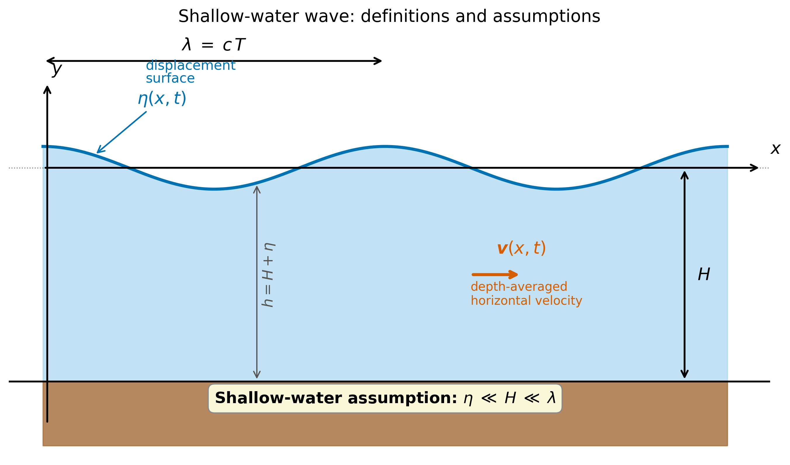— Fig. 85 Definitions for the shallow-water wave. The total water depth is \(h(x, t) = H + \eta(x, t)\), with \(H\) the equilibrium depth and \(\eta\) the surface displacement (small: \(\eta \ll H\)). The horizontal water-particle velocity \(v(x, t)\) is taken to be uniform with depth (the shallow-water approximation). The wavelength \(\lambda\) is much larger than \(H\). Reproduces the geometry of legacy slide 39.#

Notation

Symbol	Meaning	Units
\(H\)	equilibrium water depth	m
\(\eta(x, t)\)	sea-surface displacement	m
\(h = H + \eta\)	instantaneous water depth	m
\(v(x, t)\)	depth-averaged horizontal water velocity	m/s
\(\rho\)	water density	kg/m³
\(g\)	gravitational acceleration	m/s²
\(c\)	wave propagation speed	m/s
\(\lambda\)	wavelength	m
\(T\)	period	s
\(A\)	wave amplitude	m
\(J\)	tsunami run-up height	m

Assumption throughout this section: \(\eta \ll H \ll \lambda\) (linear, non-dispersive shallow-water limit).

3.2 Mass and momentum balance#

Consider a one-dimensional column of water of horizontal length \(\lambda\) (one wavelength), unit width into the page, and total depth \(h(x, t) = H + \eta(x, t)\). The mass per unit length contained in one wavelength is

(134)#\[ m_{\lambda} \;=\; \rho\,V_{\lambda} \;=\; \rho\,\lambda\,H, \]

with the approximation \(h \approx H\) since \(\eta \ll H\). The horizontal force per unit length driving the flow comes from the pressure differential across one wavelength. Hydrostatic pressure at depth gives \(\Delta p = \rho g \eta\) (the pressure under the crest exceeds the pressure under the trough by \(\rho g \eta\)), so the net horizontal force per unit length acting on the column is

(135)#\[ F \;=\; \Delta p \cdot H \;=\; \rho\,g\,\eta\,H. \]

Newton’s second law gives the acceleration of the water column,

(136)#\[ a \;=\; \frac{F}{m_{\lambda}} \;=\; \frac{\rho g \eta H}{\rho \lambda H} \;=\; \frac{g\,\eta}{\lambda}. \]

The horizontal velocity of the displaced water in time \(T\) (one period) is then \(v = aT\), so

(137)#\[ v \;=\; \frac{g\,\eta}{\lambda}\,T. \]

3.3 Mass conservation closes the system#

A second relation comes from conservation of water volume. Over one period, a horizontal mass flux of \(m_{\text{flux}} = \rho v T H\) flows past any vertical cross-section. By mass conservation this must equal the volume of water “stored” by the rising surface displacement \(\eta\) over the wavelength,

(138)#\[ \rho\,v\,T\,H \;=\; \rho\,\lambda\,\eta. \]

Substituting equation (137) for \(v\):

\[ \rho \cdot \frac{g\,\eta}{\lambda}\,T \cdot T \cdot H \;=\; \rho\,\lambda\,\eta, \qquad\Longrightarrow\qquad \frac{g\,T^2\,H}{\lambda} \;=\; \lambda, \]

(139)#\[ \Longrightarrow\quad \frac{\lambda^2}{T^2} \;=\; g\,H. \]

Since wave speed is \(c = \lambda / T\), equation (139) states the central result:

(140)#\[ \boxed{\;c \;=\; \sqrt{g\,H}\;.} \]

Key Equation — Shallow-water tsunami speed

In water of depth \(H\), a tsunami propagates at

\[ c \;=\; \sqrt{g\,H}. \]

Numerical examples for an open-ocean tsunami:

Region	\(H\) (m)	\(c\) (m/s)	\(c\) (km/h)
Pacific abyssal plain	4000	198	713
Continental shelf	200	44	159
Coastal shelf	50	22	79
Just offshore	10	9.9	36

In the open ocean the tsunami matches a commercial jet’s cruising speed. By the time it shoals onto a beach it has slowed by a factor of ~30, and by mass conservation its energy is compressed into a much shorter wavelength and much greater amplitude.

3.4 What the formula says — and what it omits#

Equation (140) makes three powerful predictions and three corresponding caveats.

Three predictions.

The wave speed depends only on water depth, not on amplitude. This means small “rumour” tsunamis travel at the same speed as catastrophic ones — and that travel-time charts can be computed from bathymetry alone, well before any source is identified.
Tsunami waves are non-dispersive. Since \(c\) does not depend on frequency or wavelength, all the spectral components in the initial displacement travel together. A pulse stays a pulse.
Tsunamis carry energy across entire ocean basins. With a wave amplitude of 1–2 m and a wavelength of 200 km, the radiation pattern is essentially geometric: amplitude decays only as \(1/\sqrt{R}\) in 2D spreading, not as \(1/R^2\) for an isotropic point source.

Three caveats.

Linearity breaks down at the coast. When \(\eta\) becomes a substantial fraction of \(H\), the leading-order \(\sqrt{g H} \to \sqrt{g(H + \eta)}\) steepens the front and the trailing edge — the tsunami transitions to a non-linear bore.
Dispersion matters for landslide-generated tsunamis. The short-wavelength components from a landslide source (\(\lambda \approx 1\)–\(10\) km) have \(H/\lambda\) not necessarily small, and shorter-period (\(T \approx 30\) s) waves move slower. The leading pulse spreads out and the long-period components arrive first.
Coriolis matters for transoceanic propagation. Across a Pacific crossing, the rotation of the Earth turns the wave path noticeably. A tsunami launched from the Aleutians does not arrive at Hilo by following a great-circle path.

4. Forward problem: propagation, shoaling, and run-up#

4.1 Open-ocean propagation: the energy-flux argument#

Consider a tsunami of amplitude \(A\) propagating in water of depth \(H\). The kinetic-energy density of the moving water column is \(\tfrac{1}{2}\rho v^2 H\); the potential-energy density of the surface displacement is \(\tfrac{1}{2}\rho g A^2\). For a linear wave, the two are equal and the total energy density per unit area is \(\rho g A^2\) (with the factor of \(\tfrac{1}{2}\) recovered by time- averaging). The energy flux carried per unit length of wavefront is then

(141)#\[ \Phi \;=\; \tfrac{1}{2}\,\rho\,g\,A^2\,c \;=\; \tfrac{1}{2}\,\rho\,g\,A^2\,\sqrt{g H}. \]

For a free-running tsunami (no dissipation, no spreading), \(\Phi\) is conserved along the propagation path. As the wave shoals from \(H_{\text{ocean}}\) to \(H_{\text{coast}}\), the speed \(c\) decreases as \(\sqrt{H}\) and the amplitude must rise to keep \(A^2 \sqrt{H}\) constant:

(142)#\[ A^2 \sqrt{H} \;=\; \text{const.} \]

Key Equation — Green’s law (shoaling amplification)

(143)#\[ \frac{A_{\text{coast}}}{A_{\text{ocean}}} \;=\; \left(\frac{H_{\text{ocean}}}{H_{\text{coast}}}\right)^{1/4}. \]

A tsunami that is 1 m tall in the open ocean (\(H = 4000\) m) reaches shallow water (\(H = 4\) m) with amplitude

\[ A_{\text{coast}} = 1\,\text{m} \times (1000)^{1/4} \approx 5.6\,\text{m}. \]

The transformation looks gentle on the page — a fourth root grows slowly with its argument — but it transforms an unobtrusive mid-ocean disturbance into a six-metre wall of water.

4.2 Run-up: the additional onshore amplification#

The amplitude predicted by Green’s law is the offshore amplitude just before the wave breaks. The run-up height \(J\) — how far up the beach the water flows — is typically 2–4× the offshore amplitude. The exact factor depends on the shoreline slope, the bay geometry, the wave period, and the local bathymetry. The 2011 Tōhoku run-up at Miyako (Tarō-chō) reached 38 m; the offshore amplitude was about 19 m, a run-up factor of 2 (Figure fig-17-tohoku-runup).

Three mechanisms enhance run-up beyond Green’s law:

Bay funnelling. A converging coastline concentrates wave energy into a smaller width as it propagates inland. The Miyako and Onagawa run-ups owe much of their severity to this geometry.
Resonance. A bay or inlet has natural seiche modes; if a tsunami’s period matches the bay’s natural period, the wave is amplified through standing-wave resonance. The 2012 Haida Gwaii tsunami at Port Alberni, BC, displayed a clear amplification at the bay’s resonant period.
Transient currents and harbour vortices. Even after the leading wave has passed, the strong inflow and outflow set up vorticity in confined harbours. Pillar Point Harbor, California, recorded 1.5 m/s currents during the 2011 Tōhoku tsunami arrival — strong enough to wreck moored vessels even with a modest wave amplitude @Lynett2012.

A two-panel figure. Top: a schematic cross-section of a tsunami propagating from deep ocean (left, depth 4000 m) onto a continental shelf (middle, depth 200 m) and then a beach (right, depth 5 m). The wave amplitude grows visibly as it shoals. Bottom: a log-log plot of amplitude amplification factor versus depth ratio, with the H to the negative one-quarter Green's law as a dashed line and the actual amplification factors observed at five Pacific stations during the 2011 Tohoku tsunami plotted as labeled points. 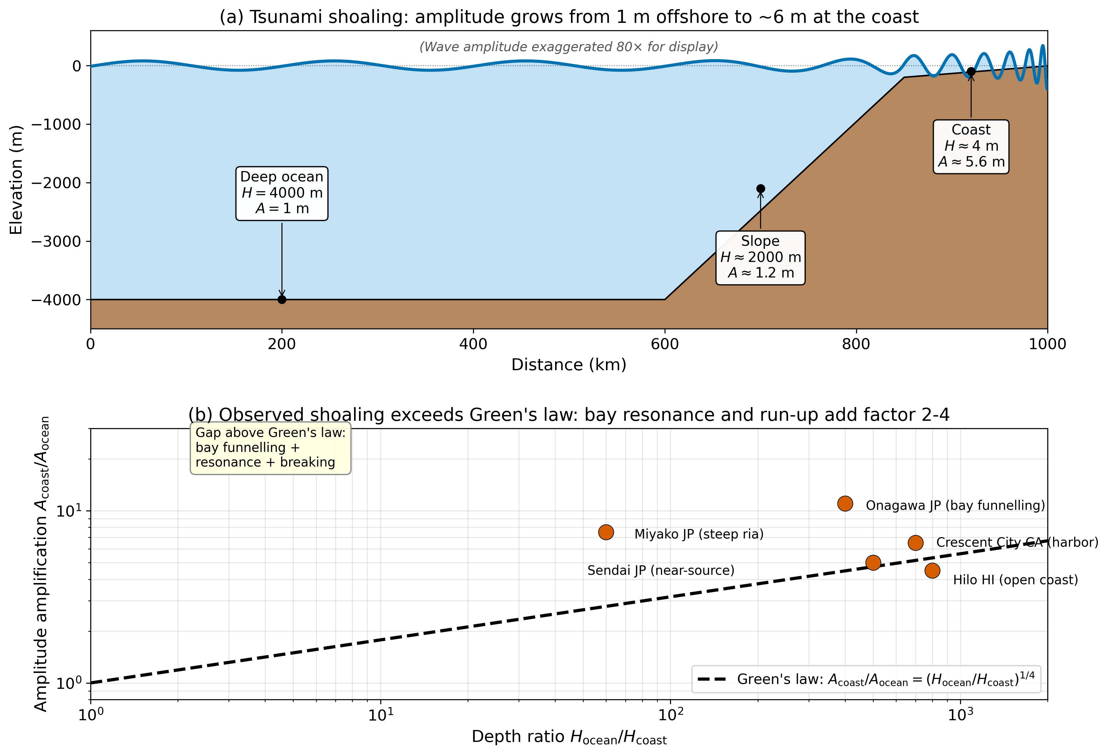— Fig. 86 Shoaling amplification of a tsunami. **Top:** as the wave moves from 4000 m water depth onto a 5 m coastal shelf, Green’s law predicts \(A_{\text{coast}}/A_{\text{ocean}} = (H_{\text{ocean}}/H_{\text{coast}})^{1/4} = (800)^{1/4} \approx 5.3\). **Bottom:** the predicted amplification versus the depth ratio is a power law of slope \(1/4\). Observed shoaling factors from the 2011 Tōhoku tsunami at five Pacific tide gauges generally fall above the line, because run-up adds an extra factor of 2–3 from bay funnelling, resonance, and non-linear breaking — all of which equation (143) ignores.#

4.3 The forward computational pipeline#

A modern tsunami forecast follows a five-step pipeline:

Estimate the source within seconds of the earthquake (USGS W-phase CMT, or seafloor pressure inversion of @Mulia2022).
Compute initial sea-surface displacement using the @Okada1985 formula and the slip distribution.
Propagate the wave by solving the shallow-water equations on a global bathymetry grid — typically using GeoClaw @LeVeque2011 (an open-source code developed at the University of Washington) or NOAA’s MOST.
Compute coastal inundation by switching to non-linear shallow-water with a moving wet-dry boundary, or by computing inundation maxima on a fine-resolution local grid (5–15 m).
Issue a warning through the Pacific Tsunami Warning Center (PTWC) and equivalent regional centres.

The first three steps are purely physics. The fourth — the inundation forecast at a specific town — is increasingly augmented with machine learning, since fully resolving inundation in real time on a 1 km grid is computationally demanding.

5. Inverse problem and observational constraints#

5.1 DART buoys: ocean-bottom pressure observations#

The NOAA DART (Deep-ocean Assessment and Reporting of Tsunamis) network @Bernard2014 deploys ~50 ocean-bottom pressure recorders at strategic locations across the Pacific and Atlantic. Each station detects pressure perturbations as small as 1 mm (equivalent to 1 mm of overlying water column) and transmits them via acoustic modem to a surface buoy and thence by satellite. A DART buoy is functionally a tsunami seismometer for the ocean — the analogue of a coastal tide gauge but located in the open ocean, where the wave is still small and roughly linear and the source inversion is more tractable.

A single DART arrival, combined with an earthquake source location, constrains the source magnitude through the @Percival2014 inversion: fit the observed pressure time series with a linear combination of precomputed Green’s functions for unit slip on each of a large set of fault patches. The Pacific tsunami warning system uses a 30-minute window of DART data to issue refined warnings — typically before the wave reaches Hawaii from a Pacific Rim source @Mungov2013.

5.2 Paleotsunami: reading the past from coastal stratigraphy#

For events older than the instrumental record — and especially for Cascadia, where no instrumental megathrust exists — the constraint on tsunami history comes from the geologic record. Two complementary archives are central.

Coastal sand layers. When a tsunami floods a coastal marsh, it deposits a sand layer on top of the underlying marsh peat or tidal mud. Subsequent sediment accumulation buries the layer. Decades later, a vertical core or trench through the marsh reveals an alternating sequence of organic-rich and sand layers — the latter each a fingerprint of a single past tsunami. Radiocarbon dating of the organic material immediately above and below each sand layer brackets the event in time. The thickness, grain size, and lateral extent of each layer constrain the wave size.

The Cascadia coast — from Vancouver Island to northern California — has yielded such layers from at least 19 tsunamis over the past 10,000 years @Atwater1996. The most recent, dated to AD 1700, has been correlated through Japanese historical records to a precise date and time of 26 January 1700, 21:00 UTC, of a \(M_W \approx 9\) Cascadia rupture: the famous “orphan tsunami” that struck Honshu without any local earthquake @Atwater2015.

Turbidite stratigraphy. A second archive lies in the deep-sea sediments beyond the continental shelf. A megathrust earthquake shakes the sediments at the head of every submarine canyon along the rupture, triggering simultaneous turbidity currents that flow down each canyon and deposit a graded sand bed at the base of the slope. @Goldfinger2012, in USGS Professional Paper 1661-F, sampled sediment cores from 19 sites along the Cascadia margin and found 13 turbidite layers in the past 10,000 years that correlate along strike — i.e., they appear at the same depth in cores from Vancouver Island to northern California. A simultaneous deposition across the entire margin requires a single source event of margin-wide extent: a megathrust rupture larger than \(M_W \approx 8.7\).

A timeline plot showing the last 10,000 years on the horizontal axis with present time on the right. Vertical bars mark the dates of identified Cascadia paleo-earthquakes inferred from coastal sand deposits and from offshore turbidites; the bars cluster into approximately 19 events with irregular intervals. Two horizontal labels indicate the average recurrence interval (~530 years) and the time elapsed since the last rupture in 1700 (>320 years). 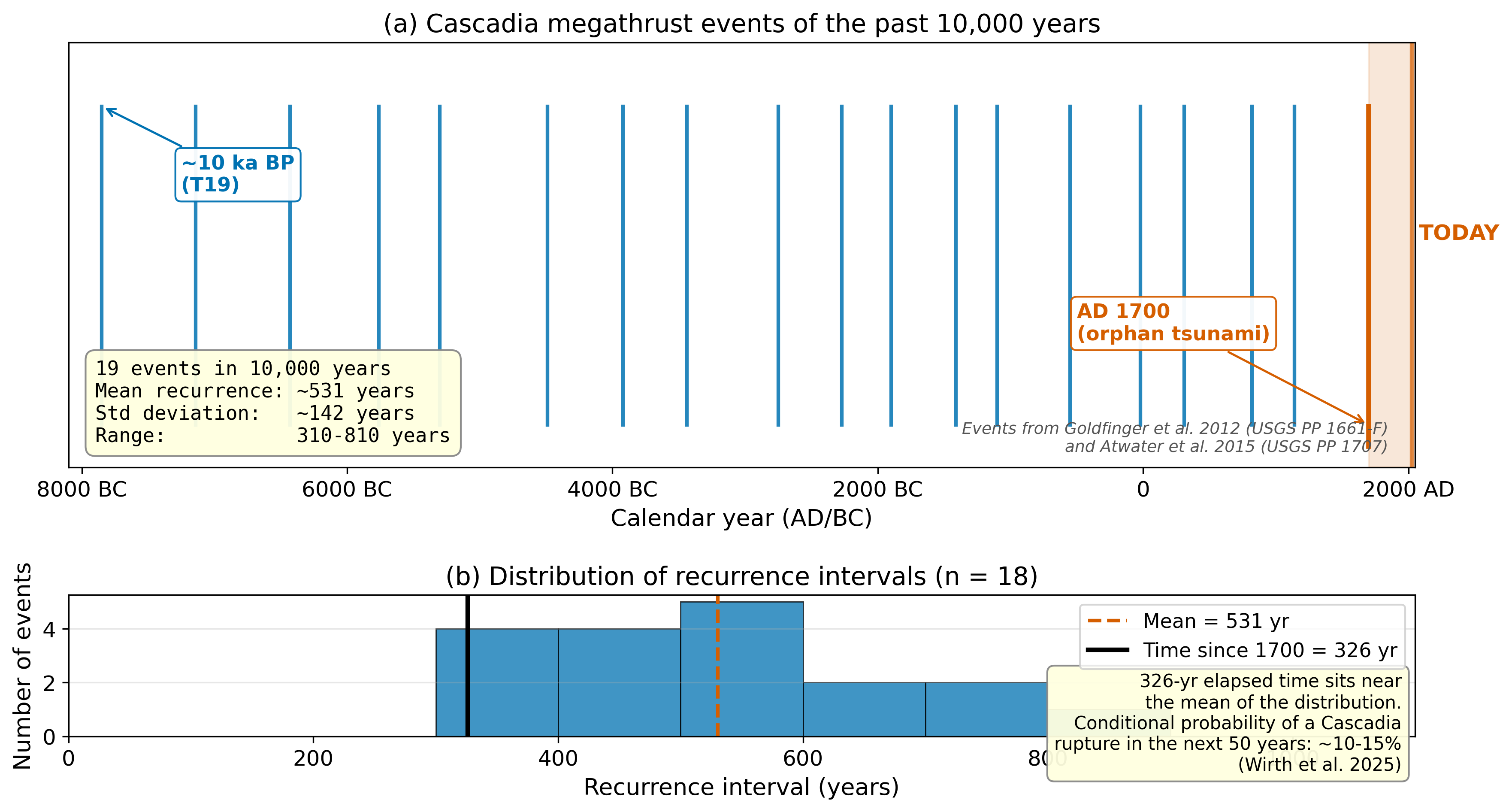— Fig. 87 The Cascadia paleoseismic record. Vertical bars mark the 19 Cascadia megathrust events of the past 10,000 years inferred from the @Goldfinger2012 turbidite chronology and corroborated by coastal-marsh sand layers @Atwater2015. The mean recurrence interval is approximately 530 years; the longest gap is ~1100 years and the shortest ~150 years. The most recent event is dated to 26 January 1700 — 326 years ago at the time of writing. Reproduces the qualitative content of legacy slides 36–38.#

The Cascadia paleoseismic record is the empirical foundation for every modern hazard estimate in the Pacific Northwest: PSHA calculations @Wirth2025, the FEMA tsunami evacuation maps, the Washington State Building Code’s \(S_a(1\text{ s})\) Cascadia values, and the 2024 WGS Tsunami Loss Estimate @WGS2024.

6. Connecting to Cascadia#

When the next Cascadia rupture occurs, three observable consequences will unfold over distinct time windows:

Time after rupture	Observable	Physics
0–3 min	Strong shaking on the coast	Crustal P-, S-, and surface waves
5–15 min	First tsunami at the coast	Local shallow-water propagation
15–60 min	Tsunami at far Pacific Northwest	Continental-shelf shoaling
4–9 hr	Tsunami arrival in Hawaii	Trans-Pacific propagation
9–14 hr	Tsunami arrival in Japan	Antipodal propagation

The most lethal window is the first one. Because the local coast lies within 100 km of the source, the tsunami arrives within ~10–20 minutes — barely time for a community to evacuate even if the warning system functions perfectly. The 2024 Washington State CSZ Tsunami Loss Estimate @WGS2024 finds that for the modelled Extended L1 \(M_W\) 9.0 scenario, evacuation success in Westport, Aberdeen, and Long Beach depends almost entirely on whether vertical-evacuation structures are in place by the time the rupture occurs.

The “natural warning” — strong, prolonged shaking — is the only warning that local communities will receive in time. Every paleoseismic and geodetic indicator points to the unique forecast that the next Cascadia tsunami will arrive within 15 minutes of the shaking that announced it.

7. Research Horizon#

Three frontiers in tsunami science illustrate where the field is moving.

Real-time tsunami inversion from offshore observations. The S-net seafloor sensor array off Japan now provides pressure measurements that capture the tsunami before it arrives at the coast. @Mulia2022 demonstrated that a deep-learning model trained on simulated S-net records can predict near-field inundation within seconds of the earthquake — a genuine improvement over the ~10-minute lag of traditional source-inversion approaches.

Bayesian tsunami forecasting at extreme scale. @Rim2025 applied 3D coupled acoustic-gravity wave simulations and full-Bayesian inversion to seafloor-pressure data, with one billion model parameters, to forecast Cascadia tsunamis in real time with quantified uncertainty — the first time a meaningful uncertainty quantification has been demonstrated at this scale.

Full physics-based simulation of Cascadia. @Wirth2025 and @Glehman2025 are now running 3D dynamic-rupture simulations constrained by paleo-subsidence and geodetic coupling, coupling them to GeoClaw inundation models, and producing the first physics-anchored ensemble of “Cascadia futures.”

8. Societal Relevance — the Cascadia evacuation conversation#

The Washington State Department of Natural Resources publishes tsunami inundation maps for every coastal community at dnr.wa.gov/tsunami. The 2024 update extends the Extended L1 \(M_W\) 9.0 scenario — the worst-case Cascadia rupture consistent with the paleoseismic constraints — to all 16 affected counties and quantifies expected losses using HAZUS @WGS2024.

The most important policy question in Pacific Northwest tsunami science is no longer “is there hazard?” — that question has been answered. It is “can we make evacuation work in 15 minutes?”

The geophysics of this lecture — \(c = \sqrt{gH}\) giving travel times, Green’s law giving amplitudes, paleoseismic recurrence giving the probability — supplies the inputs to that question. The answer requires civil engineering (vertical evacuation structures), land-use planning (residential restrictions in inundation zones), and continuous community education (the Sneaker Wave and ShakeAlert programs).

Resources for further reading:

Washington Geological Survey, Tsunamis portal: dnr.wa.gov/tsunami
NOAA Center for Tsunami Research (PMEL Seattle): nctr.pmel.noaa.gov
University of Washington Tsunami Modeling Group: depts.washington.edu/ptha
GeoClaw open-source code: clawpack.org

9. AI Literacy — Critique a generated tsunami advisory#

AI Epistemics — Critique a generated evacuation recommendation (LO-7, LO-OUT-H)

Use a generative AI assistant and submit:

“I live in Aberdeen, Washington, on the coast. A magnitude 9.0 Cascadia earthquake just happened. How long before the tsunami arrives, how high will it be, and what should I do?”

Evaluate the response against the framework of this lecture:

Does it give a travel time consistent with \(c = \sqrt{gH}\)? For Aberdeen, the source rupture is ~80–120 km offshore in water with average depth ~1500 m on the shelf. Travel time \(\approx 80\,\text{km} / \sqrt{9.81 \times 1500\,\text{m}} \approx 80\,\text{km} / (120\,\text{m/s}) \approx 11\) minutes. An answer of “an hour” or “several hours” is qualitatively wrong; an answer of “15–25 minutes” is in the right zone.
Does it apply Green’s law for amplitude? A 1 m offshore wave becomes a ~5 m offshore-shoreline wave by Green’s law and a ~10–20 m run-up at the bay head. An AI that says “a metre or so” is using free-surface (deep-ocean) amplitude inappropriately for a coastal forecast.
Does it correctly identify the only effective warning as the shaking itself? The AI should not advise the user to wait for an official warning — for a near-field Cascadia event there is not enough time. The protocol is “strong shaking lasting longer than 30 seconds → move immediately to high ground.”
Does it acknowledge uncertainty and non-uniqueness? Different rupture distributions produce different inundation patterns at different communities. The AI should reference the WGS Extended L1 model, not commit to a single number.

Submit a 250-word critique. (Lab 5 has the rubric.)

10. Concept Checks#

A submarine earthquake produces a 1 m tsunami in 4000 m water. Compute (a) the open-ocean wave speed in m/s and km/h; (b) the amplitude on a 4 m coastal shelf using Green’s law; (c) a plausible run-up height at a converging bay head, using a run-up factor of 2.5.
Two earthquakes on the Pacific Rim each have \(M_W\) 9. One is a thrust event with 25 m of vertical slip; the other is a strike- slip event with 15 m of horizontal slip on a vertical fault. Which produces the larger tsunami, and why?
Suppose a paleoseismic core through a Cascadia coastal marsh reveals five sand layers in the upper 2 m of the section. Above each layer is a thin organic-rich peat that radiocarbon-dates to roughly 320, 850, 1300, 1700, and 2200 years before present. What is the mean recurrence interval inferred from this record, what is its standard deviation, and what is the time-since-the- last-event contribution to the conditional probability of the next event in the next 50 years?
Compute the Pacific transit time of a tsunami from the Aleutians to Hilo, Hawaii. Pacific average depth is ~4280 m; great-circle distance is ~3700 km. Compare your answer to the observed transit times (~4–5 hours).

11. Connections#

This lecture is the closing piece of Module 4 (Earthquake Phenomenology). It connects backward to Lecture 17 — Ground Motions — the same Cascadia rupture, this time observed as an oceanic forcing rather than a forcing of the built environment.

It connects forward to Module 5 (Gravity), where we encounter another potential field — gravity — that is similarly governed by an integral of subsurface mass distribution. The forward and inverse problems are mathematically parallel: from observations on the surface, infer what lies beneath.

The shallow-water mathematics of §3 reappears in the geodynamics of Module 7 (mantle convection) — the dynamics of a thin layer over a rigid substrate is one of the few configurations in continuum mechanics that admits an exact, intuitive solution.


Course LOs addressed	LO-1 (sea-surface observable from rupture), LO-2 (shallow-water wave model), LO-3 (forward propagation + inverse paleoseismology), LO-4 (limits of \(c=\sqrt{gH}\)), LO-5 (GeoClaw simulations as computational forward models), LO-6 (uncertainty in inundation), LO-7 (critique of AI evacuation advice)
Learning outcomes practiced	LO-OUT-A (sketch initial uplift + propagation), LO-OUT-B (compute travel times across the Pacific), LO-OUT-C (why \(c\) depends on \(H\) but not on \(\rho\) or \(g\) in the linear regime — wait, it depends on \(g\)), LO-OUT-D (paleotsunami inverse), LO-OUT-F (which method for which question), LO-OUT-H (critique of AI tsunami forecast)
Prior lecture	Lecture 17 — Ground Motions: the Cascadia rupture as a forcing of the built environment
Next lecture	Lecture 19 — Earth’s Gravity: a different observable of mass distribution
Lab connection	Lab 5 (planned): students compute Pacific tsunami travel times from \(c = \sqrt{gH}\) and bathymetry
Discussion connection	Session 8 — Guest: Science–Society Boundary (tsunami evacuation planning, communicating risk to coastal communities)