Earth’s Magnetic Field and the Geodynamo

Earth’s Magnetic Field and the Geodynamo#

Prerequisites#

Students should be comfortable with the vector calculus introduced in the gravity module (Lectures 19–22) — in particular, the idea that a scalar potential generates a vector field by gradient, and that surface measurements can be projected onto local Cartesian components. Familiarity with the inverse-square law and with the ensemble-fit framework from gravity will transfer directly. No prior exposure to electromagnetism beyond an introductory-physics treatment of a bar magnet is required; the constitutive relation between $\mathbf{B}$, $\mathbf{H}$, and $\mathbf{M}$ is introduced from scratch in §2.

Notation reference (this lecture)

This table lists every symbol introduced in Lecture 23. Symbols marked (L23–L25) are reused unchanged in Lectures 24 and 25; symbols marked (local to L23) appear only in this lecture.

Symbol	Name	Units / notes
$\mathbf{B}$	Magnetic flux density — what a magnetometer measures (Lorentz-force field). (L23–L25)	T; nT $= 10^{-9}$ T
$\mathbf{H}$	Auxiliary magnetic field; produced by free currents alone. (L23–L25)	A m$^{-1}$
$\mathbf{M}$	Magnetisation — volume density of atomic dipole moments. (L23–L25)	A m$^{-1}$
$\mu_0$	Permeability of free space. (L23–L25)	$4\pi\times 10^{-7}$ T m A$^{-1}$
$\mu$	Material permeability: $\mu = \mu_0(1+\chi)$.	T m A$^{-1}$
$\chi$	Volume magnetic susceptibility — linear-response coefficient $\mathbf{M}=\chi\mathbf{H}$. (L23–L25)	dimensionless (SI)
$F$	Total field intensity at a station: $F =	\mathbf{B}
$\mathbf{F}$	Total-field vector at a station (same magnitude $F$).	nT
$D$	Declination — horizontal angle of $\mathbf{F}$ east of true north. (L23–L25)	degrees
$I$	Inclination — angle of $\mathbf{F}$ below horizontal. (L23–L25)	degrees
$X,\,Y,\,Z$	Local Cartesian components of $\mathbf{F}$ (north / east / down).	nT
$H_\text{horiz}$	Horizontal magnitude $H_\text{horiz} = F\cos I$ (subscripted to avoid clash with $\mathbf{H}$).	nT
$\mathbf{m}$	Magnetic dipole moment — Earth’s geomagnetic moment in L23; a buried-body moment in L25. (L23, L25)	A m$^2$
$r$, $\hat{\mathbf{r}}$	Radial distance from the dipole and its unit vector.	m, —
$\theta$	Magnetic colatitude (angle from the dipole north pole).	rad / degrees
$\lambda$	Geographic latitude (used in $\tan I = 2\tan\lambda$). (L23, L24)	degrees
$B_r,\,B_\theta$	Radial and tangential components of the dipole field.	nT
$n$	Spherical-harmonic degree (Mauersberger–Lowes spectrum).	integer
$R_n$	Power per harmonic degree of the surface field.	nT$^2$
$r_\text{CMB},\,r_\text{surf}$	Core-mantle-boundary and Earth-surface radii (3 480 km; 6 371 km).	km
$\mathbf{u}$	Outer-core fluid velocity.	m s$^{-1}$
$\eta$	Magnetic diffusivity, $\eta = 1/(\mu_0\sigma)$.	m$^2$ s$^{-1}$
$\sigma$	Electrical conductivity of liquid iron ($\sim 10^6$).	S m$^{-1}$
$R_m$	Magnetic Reynolds number, $R_m = UL/\eta$.	dimensionless
$Ro$	Rossby number, $Ro = U/(2\Omega L)$.	dimensionless
$\Omega$	Earth’s rotation rate ($7.27\times 10^{-5}$ rad s$^{-1}$).	rad s$^{-1}$
$T_C$	Curie temperature (introduced in detail in L24). (L23–L25)	°C

Conventions adopted throughout the magnetism module (L23–L25). Vectors use bold roman ($\mathbf{B}$, $\mathbf{H}$, $\mathbf{M}$); unit vectors carry a hat ($\hat{\mathbf{r}}$, $\hat{\mathbf{m}}$, $\hat{\boldsymbol\theta}$). All subscripts use upright text (\text{...}) — e.g. $H_\text{horiz}$, $\mathbf{M}_\text{rem}$, $r_\text{CMB}$ — never the older \rm form. Angles in degrees are written with the Unicode glyph (°, e.g. $I = 68.9°$) rather than ^\circ. Numbers $\geq 10\,000$ use a thin-space thousands separator (e.g. $50\,000$ nT).

1. The framing question#

A compass needle in Seattle today points 15.5° east of true north. In 1955 it pointed 22.1° east. The asphalt of Seattle-Tacoma’s main runway was repainted in 2019 to keep its name, “16R”, honest.

A pilot lining up on runway 16R at Seattle-Tacoma International Airport is flying along a heading numbered to match Earth’s magnetic field. The number “16” means the runway points along magnetic bearing 160°. That number has to be repainted every decade or two, because the magnetic field at Seattle is not static: its declination — the horizontal angle between magnetic north and true (geographic) north — has decreased from about $+22°$ in 1955 to about $+15.5°$ in 2026. KSEA’s main runway was renamed from 16L/34R to 16R/34L in 2019 to keep up with this drift.

That a planetary-scale physical quantity changes fast enough to alter aviation infrastructure is itself a clue to what the field is and where it comes from. Three observations frame this lecture:

The surface field has a dominantly dipolar geometry, with its axis tilted about 11° from the rotation axis.
The field has multiple sources — core, lithosphere, ionosphere — with very different spatial scales and physical mechanisms.
The core source — the geodynamo — is a self-sustaining magnetohydrodynamic process in the liquid outer core, and it is responsible for the dipole, the secular variation, and the polarity reversals.

Global contour map of magnetic declination D for the IGRF-13 epoch 2026.0 in a Mollweide-style projection. Solid blue contours mark positive declination (compass east of true north), dashed orange contours mark negative declination (compass west of true north), and a heavy black contour traces the agonic line D = 0. The agonic line sweeps from the western Pacific over the Asian interior down through India and the Indian Ocean, and a second branch crosses North America from the Hudson Bay through the eastern United States to the South Atlantic. Four station labels mark Seattle (D = +15.0 degrees), Anchorage (D = +14.2 degrees), London (D = +1.1 degrees), and Tokyo (D = -7.9 degrees). 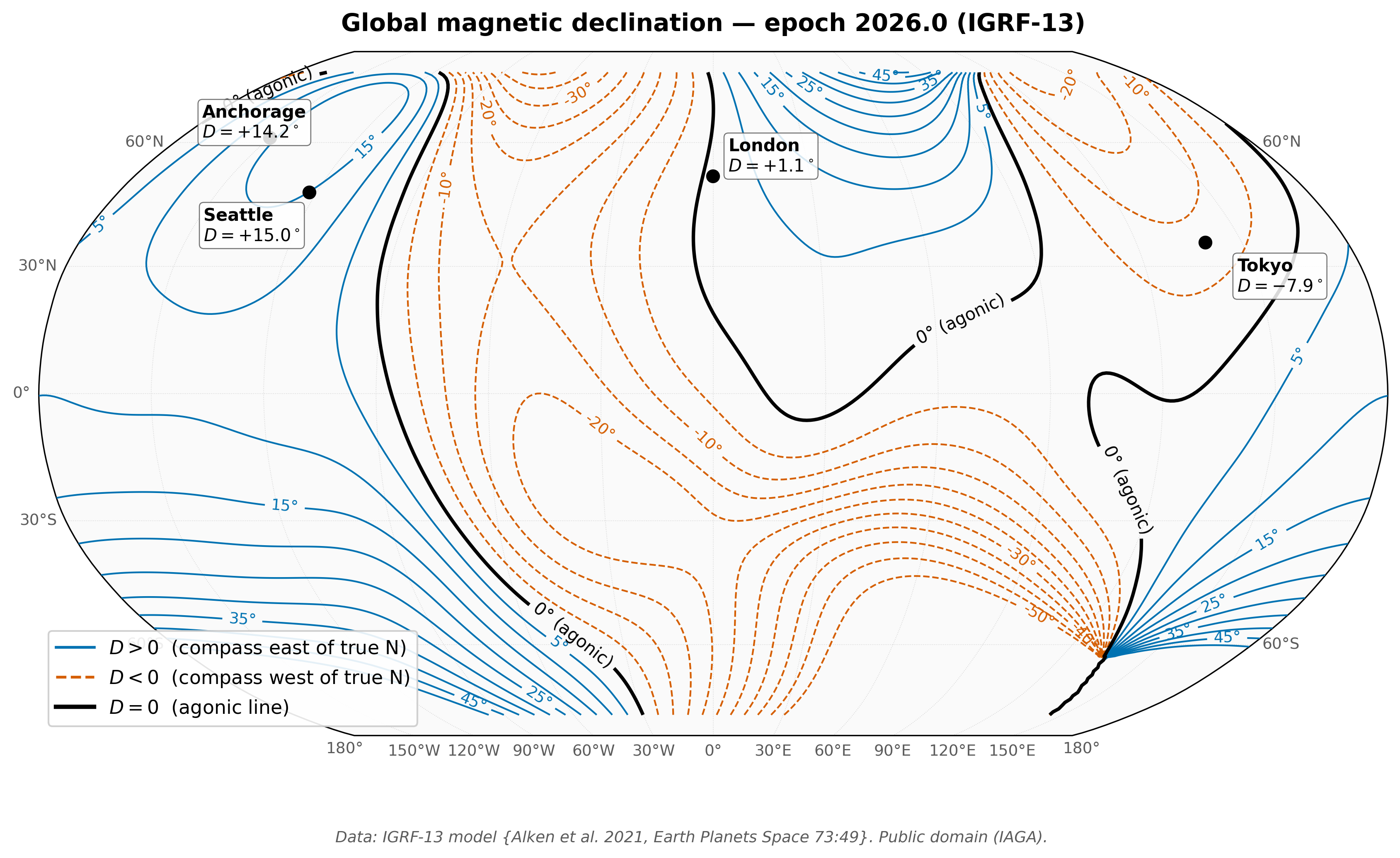— Fig. 99 Global magnetic declination $D$ for IGRF-13 epoch 2026.0 [Alken *et al.*, 2021]. Compass deviations of $\pm 30°$ or more are common; the **agonic line** $D = 0$ wanders from continent to continent and itself drifts at $\sim 0.2°$ per year (section 6). At Seattle today $D \approx +15°$ — the compass needle points $15°$ east of true north — which is why KSEA repainted runway 16R in 2019. Public domain (IAGA).#

Today’s lecture builds out (1), (2), and (3). Lectures 24 and 25 take the crustal component of the surface field — the static remnant in (2) — and turn it into a tool for imaging the lithosphere.

2. The fields: $\mathbf{B}$, $\mathbf{H}$, $\mathbf{M}$, and $\chi$#

Before we can write down the dipole or talk about the geodynamo, we need three vector fields and one constitutive relation.

2a. The three fields#

There are three vector quantities that get loosely called “the magnetic field” in informal usage. They are distinct, they have different units, and they are not interchangeable.

Magnetic flux density $\mathbf{B}$, with SI units of tesla ($1\,\text{T} = 1\,\text{kg}\,\text{s}^{-2}\,\text{A}^{-1}$). This is what a magnetometer actually measures: the force per unit current per unit length on a wire (the Lorentz force law $\mathbf{F} = q\mathbf{v}\times\mathbf{B}$). $\mathbf{B}$ is what is sometimes called the magnetic field; in geomagnetism the surface scalar value is denoted $F = |\mathbf{B}|$ and quoted in nanoteslas ($1\,\text{nT} = 10^{-9}\,\text{T}$). At Earth’s surface $F$ ranges from $\sim 25\,000$ nT near the magnetic equator to $\sim 65\,000$ nT near the poles.
Auxiliary field $\mathbf{H}$, with SI units of ampere per metre ($\text{A m}^{-1}$). Historically $\mathbf{H}$ was the “magnetic field strength” and $\mathbf{B}$ the “magnetic induction” — modern texts reverse the emphasis. $\mathbf{H}$ is what you would calculate from the free electric currents alone via Ampère’s law $\nabla \times \mathbf{H} = \mathbf{J}_{\text{free}}$; it ignores the contribution of bound atomic currents (magnetised matter). In a vacuum, $\mathbf{H}$ and $\mathbf{B}$ are proportional: $\mathbf{B} = \mu_0 \mathbf{H}$, with $\mu_0 = 4\pi \times 10^{-7}\,\text{T m A}^{-1}$ the permeability of free space.
Magnetisation $\mathbf{M}$, also with SI units of ampere per metre ($\text{A m}^{-1}$). This is the volume density of magnetic dipole moments carried by the material: $\mathbf{M} = (1/V)\sum_i \mathbf{m}_i$. In free space, $\mathbf{M} = 0$. Inside a rock, $\mathbf{M}$ is the geophysically interesting quantity — it is what carries the signal of crustal magnetism.

2b. The constitutive relation#

The three fields are tied together by

(174)#\[ \boxed{\;\mathbf{B} = \mu_0\!\left(\mathbf{H} + \mathbf{M}\right).\;} \]

Equation (174) is a definition — it says how the total flux density $\mathbf{B}$ is the sum of two contributions: the field $\mu_0 \mathbf{H}$ produced by free currents (e.g. the geodynamo’s currents in the core) and the field $\mu_0 \mathbf{M}$ produced by the bound atomic currents inside magnetised matter (e.g. magnetite grains in a basalt). It holds everywhere — in vacuum (where $\mathbf{M} = 0$), in the outer core (where $\mathbf{M} \approx 0$ because liquid iron is above its Curie temperature), and in crustal rocks (where $\mathbf{M}$ can be substantial).

In a linear, isotropic medium the magnetisation is proportional to the applied field through the dimensionless magnetic susceptibility $\chi$:

(175)#\[ \mathbf{M} = \chi \, \mathbf{H}. \]

Substituting (175) into (174):

(176)#\[ \mathbf{B} = \mu_0 \left(1 + \chi\right) \mathbf{H} = \mu \, \mathbf{H}, \]

where $\mu = \mu_0(1+\chi)$ is the permeability of the material. For most crustal rocks $\chi \ll 1$ (typically $10^{-5}$ to $10^{-2}$), so $\mathbf{B} \approx \mu_0 \mathbf{H}$ to better than one percent and the distinction between $\mathbf{B}$ and $\mu_0 \mathbf{H}$ matters only inside high-$\chi$ minerals like magnetite. For practical geomagnetism we therefore work with $\mathbf{B}$ — the directly measured quantity — and reserve $\mathbf{H}$ for situations where we must separate free from bound currents.

Two side-by-side schematic blobs of matter showing the linear-media constitutive relation. The left panel labelled Diamagnet (chi less than zero) shows an applied field H pointing upward and a magnetisation M pointing downward, with internal atomic dipoles aligned opposite to H. The right panel labelled Paramagnet (chi greater than zero) shows H pointing upward and M also pointing upward, with internal atomic dipoles aligned with H. Below the two panels the chain of equalities B equals mu-zero times (H plus M) equals mu-zero times (H plus chi H) equals mu-zero times (1 plus chi) times H equals mu times H is written out, with labels identifying the applied field, the material response, and the permeability mu equals mu-zero times (1 plus chi). 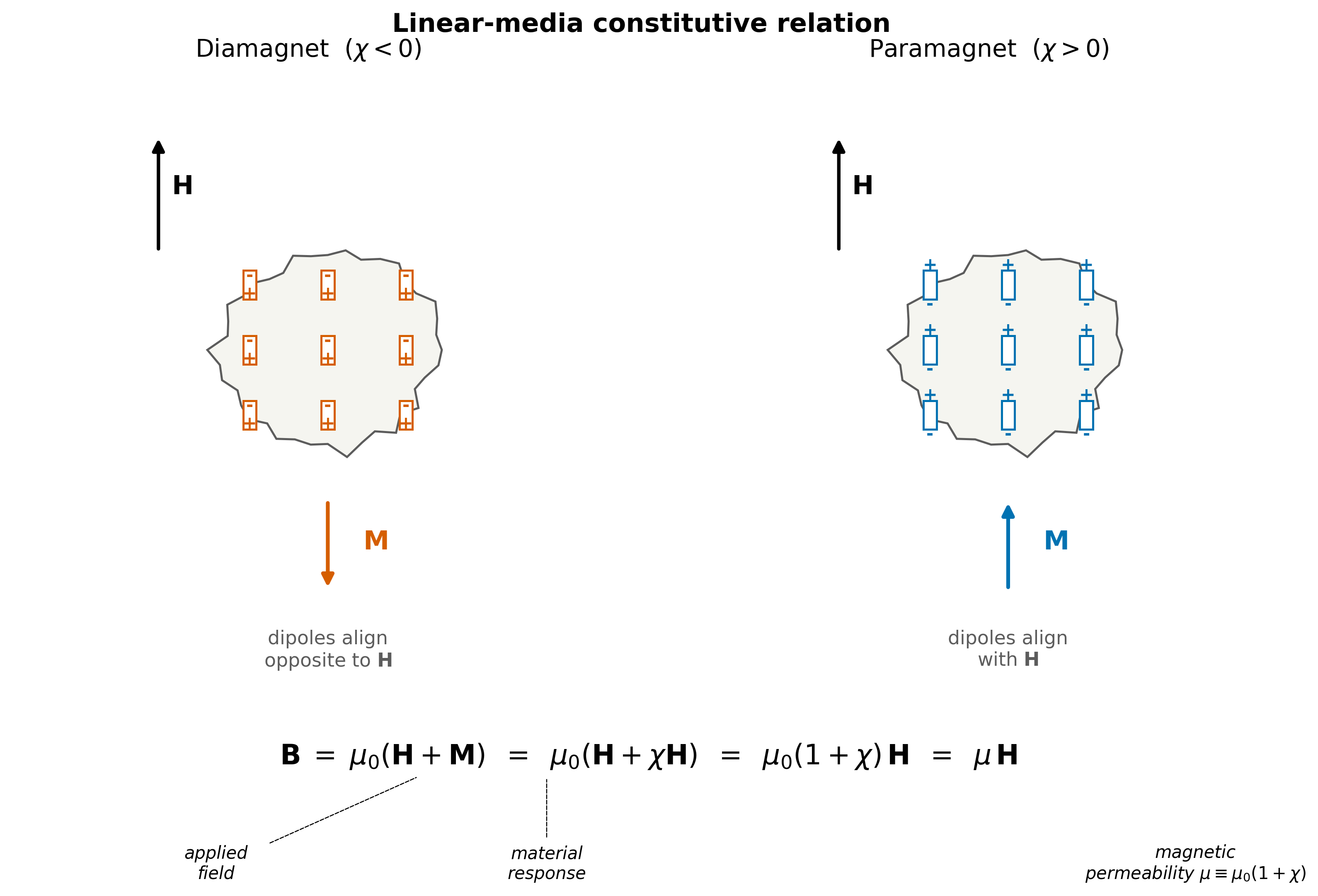— Fig. 100 The linear-media constitutive relation $\mathbf{B} = \mu_0(\mathbf{H}+\mathbf{M}) = \mu_0(1+\chi)\mathbf{H} = \mu\mathbf{H}$ visualised for two regimes. In a **diamagnet** ($\chi < 0$) the induced atomic dipoles align *opposite* to the applied $\mathbf{H}$, so $\mathbf{M}$ points opposite to $\mathbf{H}$ and the medium slightly weakens the total $\mathbf{B}$ inside the body. In a **paramagnet** ($\chi > 0$) the dipoles align *with* $\mathbf{H}$ and the medium slightly enhances $\mathbf{B}$. The third regime — ferro/ferrimagnetic, where $\mathbf{M}$ can persist after $\mathbf{H}$ is removed — is the subject of Lecture 24.#

Why two field symbols at all?

Why do we need $\mathbf{B}$ and $\mathbf{H}$ when they differ by less than one part in $10^5$ outside ferromagnetic minerals? The answer is that the two enter the fundamental equations of magnetism in different ways. Ampère’s law is naturally written in terms of $\mathbf{H}$ because it isolates the free-current source; the Lorentz force law is naturally written in terms of $\mathbf{B}$ because what acts on a moving charge is the total flux density. When we discuss the dipole in §3 we will use $\mathbf{B}$ throughout, but the constitutive relation (174) is what bridges to the induced magnetisation $\mathbf{M} = \chi\mathbf{H}$ that we will need in Lectures 24 and 25.

The rock-magnetic content of (175) — what makes $\chi$ small for quartz and large for magnetite, and how rocks acquire a remanent (i.e. non-induced) magnetisation in the absence of any applied field — is the subject of Lecture 24. Here we keep $\mathbf{M} = 0$ outside the Earth and focus on $\mathbf{B}$ at the surface.

3. The dipole and the $(D, I, F)$ system#

Earth’s surface magnetic field at most non-equatorial locations is, to first order, the field of a centred magnetic dipole tilted about 11° from the rotation axis. The dipole accounts for roughly 90% of the surface field’s power.

3a. The dipole field#

The magnetic flux density of a point dipole with moment $\mathbf{m}$ (units $\text{A m}^2$), measured at position $\mathbf{r}$ relative to the dipole, is

(177)#\[ \mathbf{B}(\mathbf{r}) = \frac{\mu_0}{4\pi}\,\frac{3(\mathbf{m}\cdot\hat{\mathbf{r}})\hat{\mathbf{r}} - \mathbf{m}}{r^3}. \]

In spherical polar coordinates aligned with the dipole axis (so $\theta$ is the colatitude measured from the north pole of the dipole), the radial and tangential components are

(178)#\[ B_r = \frac{\mu_0}{4\pi}\,\frac{2 m \cos\theta}{r^3}, \qquad B_\theta = \frac{\mu_0}{4\pi}\,\frac{m \sin\theta}{r^3}. \]

Meridional cross-section of an idealised magnetic dipole drawn in Earth's true polarity. A circular boundary in the centre encloses a vertical orange arrow labelled m pointing downward, from the magnetic south pole (top, labelled "geographic N / magnetic S") to the magnetic north pole (bottom, labelled "geographic S / magnetic N"). A dense family of dipole field lines (curved black streamlines with arrowheads) emerges from the magnetic north pole at the bottom, loops outward through space, and re-enters at the magnetic south pole at the top. At one surface point in the lower-right quadrant, the radial component B-sub-r is drawn as a blue arrow pointing outward and the tangential component B-sub-theta is drawn as an orange arrow tangent to the surface, illustrating the polar decomposition. A small inset box reproduces the two equations B-sub-r equals (mu-zero over four pi) times m times two cosine theta over r cubed, and B-sub-theta equals (mu-zero over four pi) times m times sine theta over r cubed. 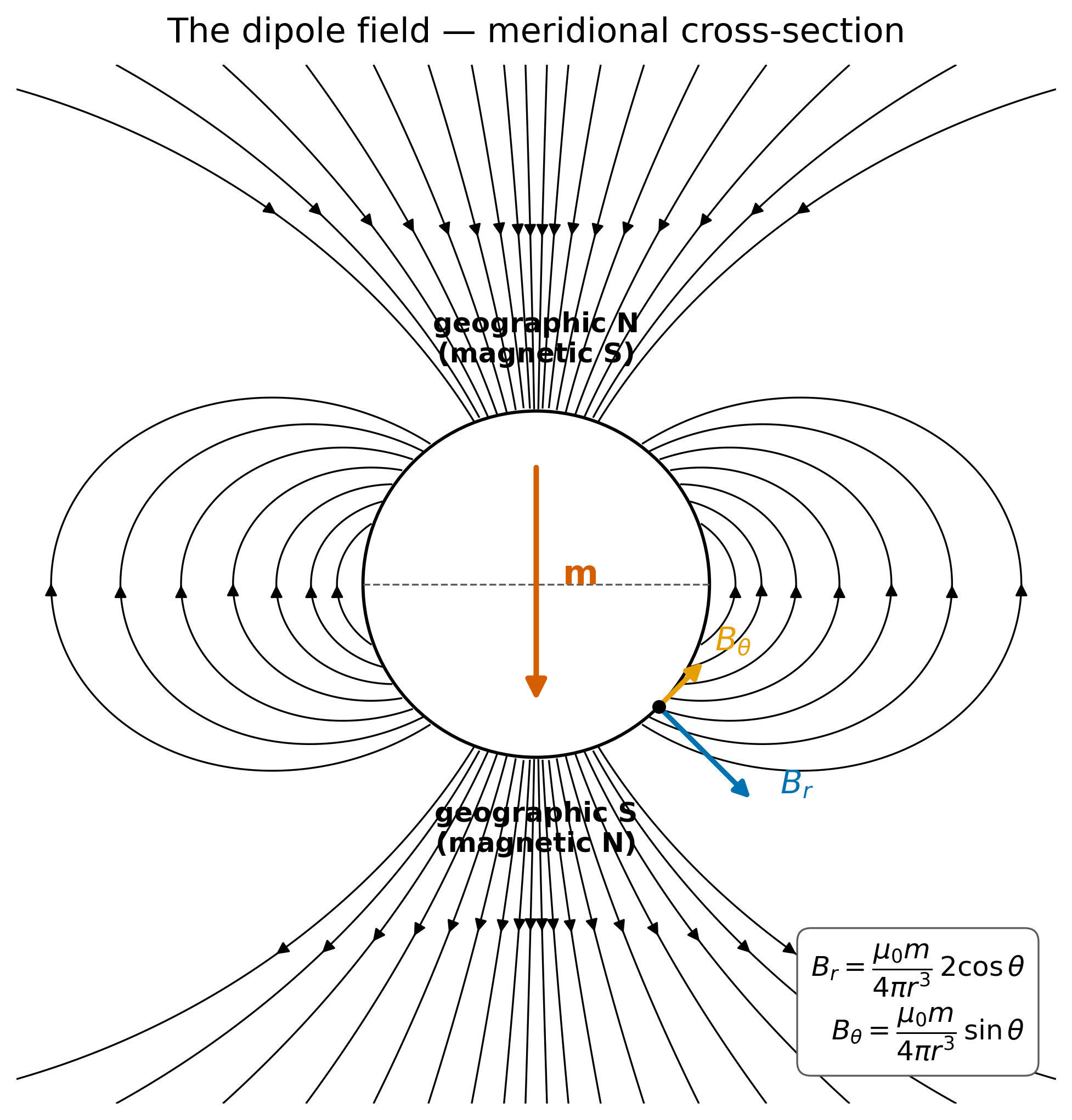— Fig. 101 The meridional field of an idealised magnetic dipole, drawn in **Earth’s true polarity**: the geographic North Pole hosts the *magnetic south* pole and the geographic South Pole hosts the *magnetic north* pole. This is why the north end of a compass needle is attracted toward geographic North — opposite poles attract. The dipole moment $\mathbf{m}$ therefore points from the geographic north toward the geographic south. The polar decomposition into $B_r$ and $B_\theta$ is marked at a representative surface point. The field falls off as $1/r^3$, and at any latitude $|B_r| = 2 |B_\theta| \cot\theta$ — the factor of 2 that returns immediately as $\tan I = 2\tan\lambda$.#

Two features matter for what follows:

The field falls off as $1/r^3$ — much faster than the gravitational $1/r^2$. This is why the surface field is dominated by the deepest, longest-wavelength contributions and why short-wavelength crustal anomalies attenuate so quickly with altitude.
At any latitude, the radial component is twice the tangential component: $B_r / B_\theta = 2 \cot\theta$. That factor of 2 will return immediately as the famous $\tan I = 2\tan\lambda$ relation.

3b. The $(D, I, F) \leftrightarrow (X, Y, Z)$ system#

At any surface station, the field is fully described by three numbers — the declination $D$, the inclination $I$, and the total intensity $F$ — or equivalently by the three components in a local Cartesian frame with $X$ pointing to true north, $Y$ pointing east, and $Z$ pointing downward:

(179)#\[ X = F \cos I \cos D, \qquad Y = F \cos I \sin D, \qquad Z = F \sin I. \]

Here $D$ is positive when the horizontal component points east of true north, and $I$ is positive when the field points into the ground, as is the case throughout the northern hemisphere at non-equatorial latitudes. The horizontal magnitude is $H_\text{horiz} = F\cos I$ (subscripted to avoid collision with the auxiliary field $\mathbf{H}$ of §2).

Two-panel figure showing the geomagnetic field at Seattle in 2026. Panel a is a map view looking downward with X (true north) along the vertical axis and Y (east) along the horizontal axis. A blue arrow labelled H (horizontal field) is rotated 15.5 degrees east of X, marking the declination D. Tick marks indicate X equals 18351 nanotesla and Y equals 5089 nanotesla. Panel b is a side view showing the horizontal line at the top, the vertical Z (down) axis, the horizontal blue component H equals F cosine I equal to 19044 nanotesla, the vertical green component Z equals F sine I equal to 49353 nanotesla, and the total-field orange vector F at inclination I equal to 68.9 degrees below horizontal. 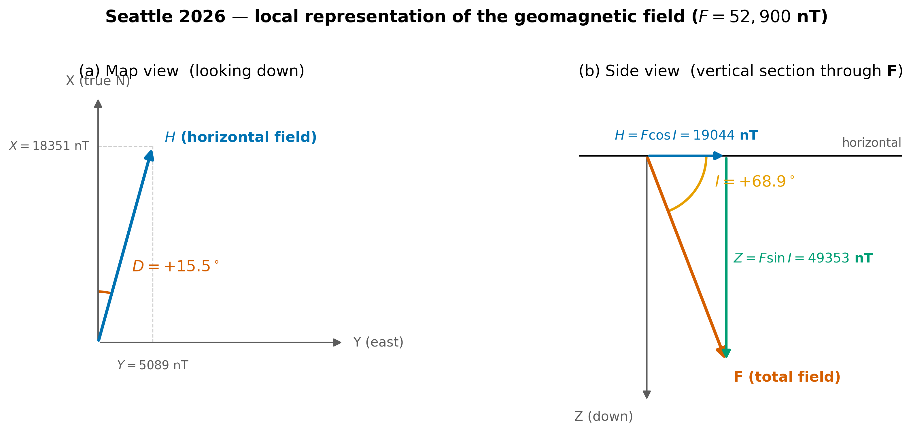— Fig. 102 The geomagnetic field at Seattle in 2026 decomposed into station coordinates. **Panel (a)** is the map view: the horizontal field $H_\text{horiz}$ (blue arrow) lies in the plane and is tilted by declination $D = +15.5°$ east of true north, giving Cartesian components $X = 18\,351$ nT (true north) and $Y = 5\,089$ nT (east). **Panel (b)** is the side view: the total field $\mathbf{F}$ (orange) lies below horizontal at inclination $I = +68.9°$, so it decomposes into a horizontal component $H_\text{horiz} = F\cos I = 19\,044$ nT and a downward component $Z = F\sin I = 49\,353$ nT. Values from IGRF-13 [Alken *et al.*, 2021].#

Worked example: Seattle 2026 station components

For Seattle (47.65° N, 122.30° W) in 2026, the IGRF-13 model gives $D = +15.5°$, $I = +68.9°$, $F = 52\,900$ nT. Applying (179):

$X = 52\,900 \cdot \cos(68.9°)\cdot \cos(15.5°) = 18\,300$ nT (toward true north)
$Y = 52\,900 \cdot \cos(68.9°)\cdot \sin(15.5°) = 5\,070$ nT (toward east)
$Z = 52\,900 \cdot \sin(68.9°) = 49\,360$ nT (downward)

The horizontal component $H_\text{horiz} = 19\,000$ nT is small compared with the vertical $Z = 49\,400$ nT: at Seattle’s latitude the field is strongly inclined, and a compass needle — which responds only to the horizontal component — is correspondingly weak.

3c. The geocentric axial dipole and $\tan I = 2 \tan\lambda$#

When we assume the dipole axis coincides with the rotation axis — the geocentric axial dipole (GAD) model, exact only after averaging over $\gtrsim 10\,000$ years of secular variation — the colatitude $\theta$ becomes $90° - \lambda$, where $\lambda$ is the geographic latitude. The local inclination $I$ is the angle between the total field and the horizontal, equivalent to the angle between $\mathbf{B}$ and $\hat{\boldsymbol\theta}$. From (178):

(180)#\[ \tan I \;=\; \frac{B_r}{B_\theta} \;=\; 2 \cot\theta \;=\; 2 \tan\lambda. \]

Equation (180) is the paleo-latitude relation that Lecture 24 inverts to recover the latitude at which a rock cooled. The factor of 2 is the same factor we noted under (178) — there is nothing in (180) beyond dipole geometry. Lecture 24 §8 applies it to the Eocene Crescent Formation to reconstruct the rotation of Siletzia.

4. Three sources of the surface field#

The dipole geometry of §3 is the shape of the field at the surface. Where the field actually comes from is a different question, and the answer is that the surface field is the sum of three contributions produced by three different physical processes at three different depths.

A half-Earth cross-section showing the three principal sources of the geomagnetic field in their physical context. The deep interior is shown with a small bright orange inner core, a yellow-orange outer core containing curved arrows that represent turbulent convection (the geodynamo), a brown mantle, and a thin bold blue band at the top representing the magnetised lithosphere with small white arrows indicating remanent magnetisation directions that vary in orientation. Above the surface a pale blue band represents the ionosphere, marked with curved horizontal arrows that depict electric currents flowing in the conducting upper atmosphere. Dashed grey curves on the right side trace dipole field lines emerging from the Earth. Three labelled callout boxes identify Source 1 (Core, geodynamo) with its depth range 2900 to 5150 km and wavelengths longer than 3000 km, Source 2 (Lithosphere, crust) in the upper 30 km with wavelengths from 400 to 3000 km, and Source 3 (Ionosphere or magnetosphere) at 80 to 500 km altitude with a broad spectrum that is time-varying on timescales of seconds to days. 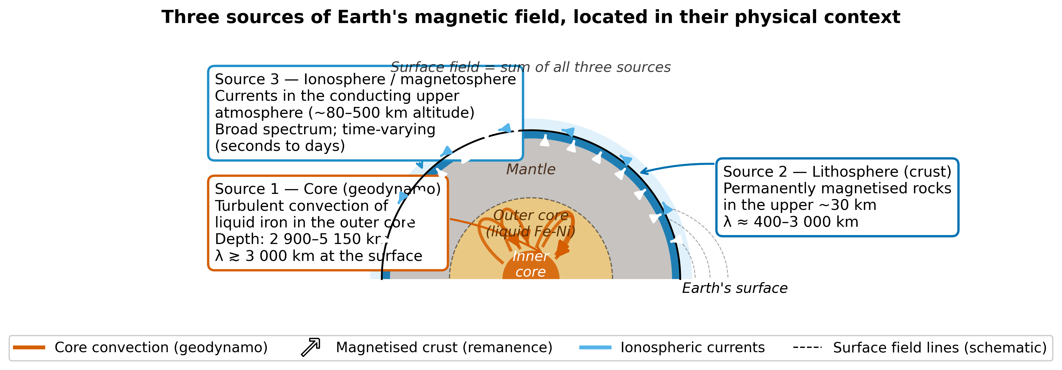A label at the top reads "Surface field equals sum of all three sources." — Fig. 103 The three sources of Earth’s magnetic field. **Source 1 — the core (geodynamo)** lies between 2 900 km and 5 150 km depth, where turbulent convection of liquid iron generates the *main field*. **Source 2 — the magnetised lithosphere** lies in the upper $\sim 30$ km of the crust. **Source 3 — the ionosphere and magnetosphere** sit above the surface ($\sim 80$–$500$ km altitude). The surface field at any station is the *sum* of all three.#

Source	Depth/altitude	Wavelength	Time scale	Surface amplitude
Core (geodynamo)	2900–5150 km depth	$\gtrsim 3\,000$ km ($n \lesssim 13$)	decades–millennia	25 000–65 000 nT
Lithosphere (crust)	0–30 km depth	400–3000 km ($n \sim 16$–$100$)	static (geological)	10–1000 nT
Ionosphere / magnetosphere	80–500 km altitude	broad	seconds–days	1–500 nT (storm)

The three sources occupy non-overlapping spatial-wavelength regimes, and that separation is what allows them to be untangled in a single power spectrum.

Meridional schematic of Earth's magnetosphere shown in cross-section with the Sun on the left and the magnetotail trailing to the right. The Sun is drawn as a small yellow disk on the far left. An orange family of solar-wind streamlines flows from left to right; on encountering the magnetosphere they sharply deflect at a dashed yellow curve labelled bow shock and then drape around a solid blue boundary labelled magnetopause. Behind Earth (a small blue disk near the centre) the field lines stretch into a long horizontal magnetotail on the right. Two pink crescents inside the magnetosphere indicate the Van Allen radiation belts, and a few internal black field lines depict the dipole geometry that becomes the surface field. 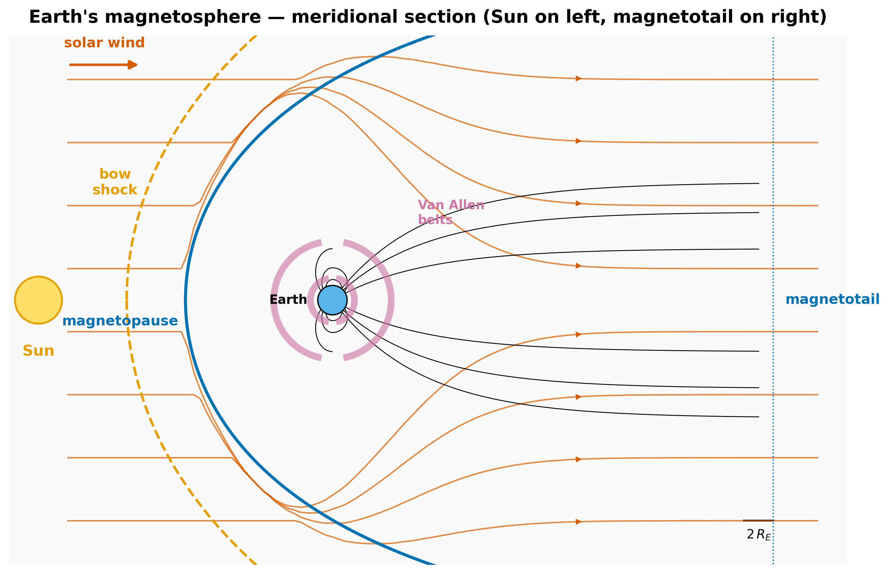— Fig. 104 The magnetosphere in meridional section. The **solar wind** (orange) is deflected by Earth’s dipole field, forming a **bow shock** upstream and a **magnetopause** that bounds the cavity carved out of the interplanetary plasma. The **magnetotail** stretches downstream for hundreds of Earth radii. Currents flowing in this system — chiefly the ionospheric Sq current at $\sim 100$ km altitude and the magnetospheric ring current at $\sim 4 R_E$ — produce the time-varying external field (Source 3) that adds to the surface signal on diurnal-to-storm timescales.#

Log-log plot of magnetic-field power per spherical-harmonic degree R_n in units of nT-squared as a function of degree n from 1 to 110. A steeply decreasing solid blue line labelled "Core (geodynamo)" falls from about 10^10 nT-squared at n=1 to below 10^-1 at n=45. A dashed orange line labelled "Crust / lithosphere" rises from near zero at n=14 to a plateau of about 50 nT-squared between n=20 and n=60, then decays slowly. A dotted green horizontal line at about 4 nT-squared marks the ionospheric external floor. The grey total-observed curve follows the core line at low n and the crust line at high n. A grey shaded region between n=13 and n=16 is labelled "core-to-crust transition". The top axis shows the approximate horizontal wavelengths in km corresponding to selected n values. 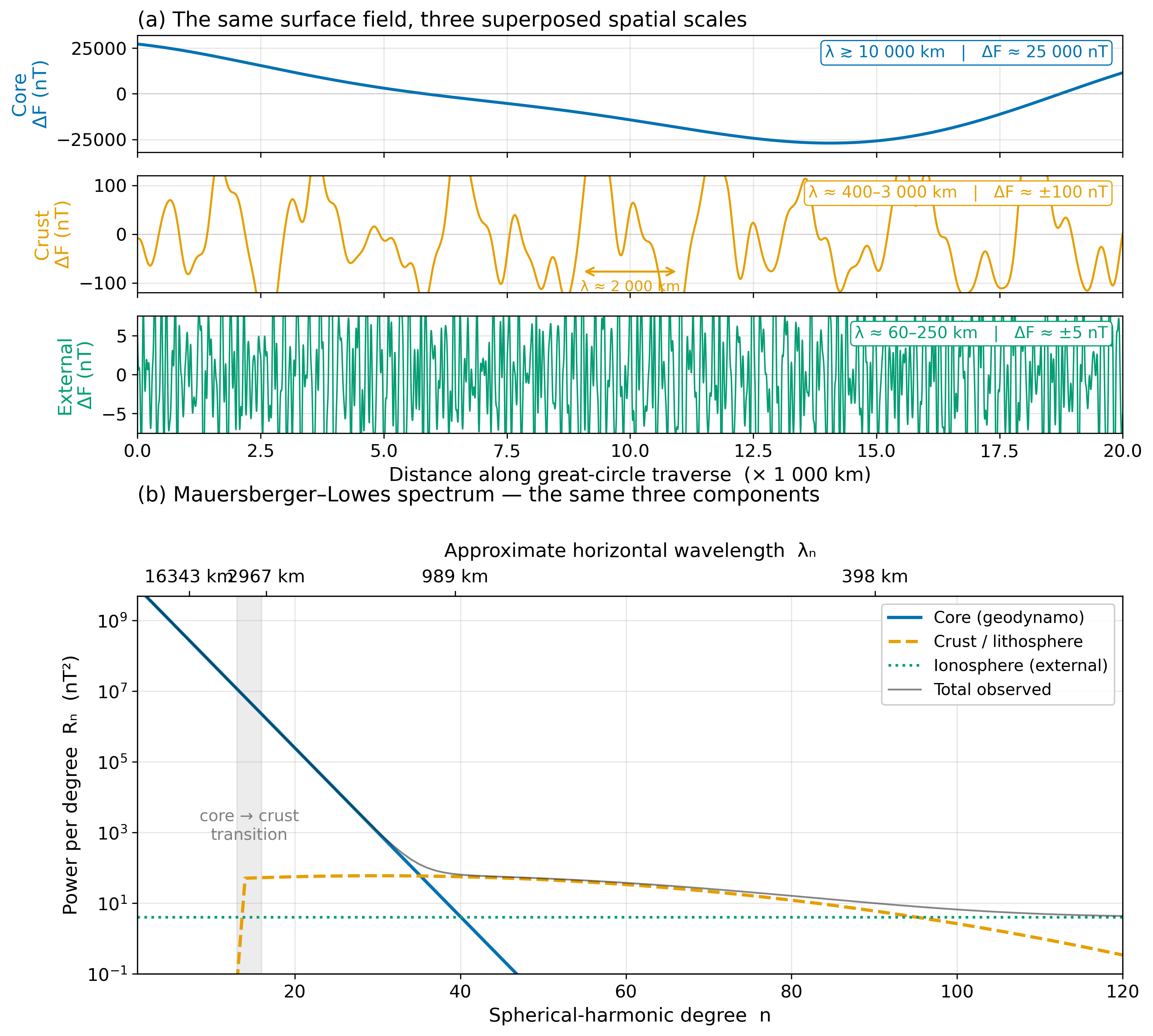— Fig. 105 The Mauersberger–Lowes power spectrum of Earth’s magnetic field at the surface. The three principal sources occupy non-overlapping wavelength regimes — the core dominates $n \le 13$, the crust dominates $n \gtrsim 16$, and the ionosphere contributes a roughly degree-independent floor. After [Maus, 2008].#

The choice of survey scale is, in effect, a choice of which source to keep and which to filter out. A satellite mission averaging over hundreds of kilometres samples the core field; a continental-scale aeromagnetic compilation isolates the lithosphere; a high-resolution ground survey along a road traverse resolves individual crustal bodies. Lectures 24 and 25 use Source 2 as signal; for the rest of today Source 1 is the signal.

5. The geodynamo#

The dominant source of the surface field is the geodynamo: self-sustaining turbulent convection of electrically conducting liquid iron in the outer core, between approximately 2 900 km and 5 150 km depth. This section unpacks the physics in four pieces — the energy source, the magnetohydrodynamic mechanism, the role of rotation, and the surface signature.

5a. The energy source#

The outer core is convectively unstable for two reasons:

Thermal buoyancy. Heat leaks from the inner-core boundary into the lower mantle at a rate of $\sim 5$–$15\,\text{TW}$ — comparable to the total radiogenic-plus-secular cooling budget of the silicate Earth.
Compositional buoyancy. As the inner core slowly freezes (radius growing by $\sim 1$ mm yr$^{-1}$), light elements (S, O, Si) are rejected into the overlying liquid. The chemically lighter residual fluid rises, releasing potential energy.

These two buoyancy sources drive convection that is vigorous by geophysical standards — characteristic velocities of $\sim 0.5$ mm s$^{-1}$ ($\sim 15\,\text{km yr}^{-1}$) — but slow by laboratory MHD standards.

5b. The MHD mechanism#

A moving conductor in a magnetic field induces an electric current; that current in turn produces a magnetic field. The closure of this loop — flow generates field that reacts back on the flow — is the magnetohydrodynamic (MHD) dynamo mechanism. The governing equation in the kinematic limit is the magnetic induction equation:

(181)#\[ \frac{\partial \mathbf{B}}{\partial t} = \nabla \times (\mathbf{u}\times\mathbf{B}) + \eta\,\nabla^2 \mathbf{B}, \]

where $\mathbf{u}$ is the fluid velocity and $\eta = 1/(\mu_0 \sigma)$ is the magnetic diffusivity ($\sigma$ is the electrical conductivity of liquid iron, $\sim 10^6\,\text{S m}^{-1}$). The two terms compete: advection by the flow stretches and bends field lines (sustaining $\mathbf{B}$), while ohmic diffusion smooths them out (destroying $\mathbf{B}$). Their ratio is the magnetic Reynolds number

\[ R_m = \frac{U L}{\eta} \sim \frac{(5\times 10^{-4}\,\text{m s}^{-1})(2\times 10^6\,\text{m})}{1\,\text{m}^2\,\text{s}^{-1}} \sim 10^3, \]

far above the dynamo threshold ($R_m \sim 10$–$100$). Earth’s core is comfortably in the regime where flow can sustain a field against ohmic decay. (Without continuous regeneration the core field would decay in $\sim 20\,000$ years.)

5c. Rotation and the tangent cylinder#

What distinguishes the geodynamo from a generic stirred conductor is rotation. The Coriolis force dominates inertia in the outer core (the Rossby number $Ro = U/(2\Omega L) \sim 10^{-6}$), and the Taylor–Proudman theorem then constrains the slow component of the flow to be invariant along the rotation axis: $\partial \mathbf{u}/\partial z \approx 0$.

This has a striking geometrical consequence. Picture the imaginary cylinder coaxial with the rotation axis whose radius equals the inner-core radius — the tangent cylinder (Fig. 103). Fluid inside the tangent cylinder cannot cross from the northern to the southern hemisphere without going through the solid inner core; fluid outside the tangent cylinder can. The two regions therefore convect with different efficiencies and produce distinguishable surface fingerprints. Numerical geodynamo simulations consistently produce flux concentrations clustered at high latitude just inside the tangent cylinder — and high-latitude flux lobes are exactly what Swarm satellite maps see at the core-mantle boundary.

5d. From core flow to surface dipole#

The field that emerges from the core-mantle boundary at $r = 3\,480$ km is filtered by depth on its way to the surface at $r = 6\,371$ km. Short spatial wavelengths attenuate as $(r_\text{CMB}/r_\text{surf})^{n+2}$ (a consequence of the harmonic Laplace equation in spherical coordinates): at $n = 13$ the attenuation is a factor of 18; at $n = 30$ it is a factor of $5\times 10^3$. The surface signature of the geodynamo is therefore dominated by long-wavelength structure — exactly the dipole-rich, $n \le 13$ part of the Mauersberger–Lowes spectrum in Fig. 105. The “Earth is a dipole” approximation that runs through every undergraduate geophysics course is a consequence of this depth filter; the geodynamo itself produces a much more complicated, time-varying field at the core-mantle boundary.

6. Secular variation, jerks, and reversals#

The geodynamo flows on timescales of years to millennia, so the surface field drifts. The drift — secular variation — is recorded at every magnetic observatory on Earth.

The recent history at Seattle (Fig. 106) tells the story through three quantities: declination $D$ dropped from about $+22°$ in 1955 to $+15.5°$ in 2026; inclination $I$ dropped from 71° to 68.9°; total intensity $F$ fell by about 3 000 nT over the same seven decades.

Three stacked line plots sharing an x-axis from 1955 to 2026 in years. The top plot is declination in degrees east of north, dropping from +22.1 degrees in 1955 to +15.5 degrees in 2026 with the endpoints annotated. The middle plot is inclination in degrees, dropping from 71 degrees to 68.9 degrees. The bottom plot is total intensity F in nanoteslas, dropping from about 56 000 nT to 52 900 nT, with a double-headed arrow on the right side annotating "delta F is approximately 3080 nT". 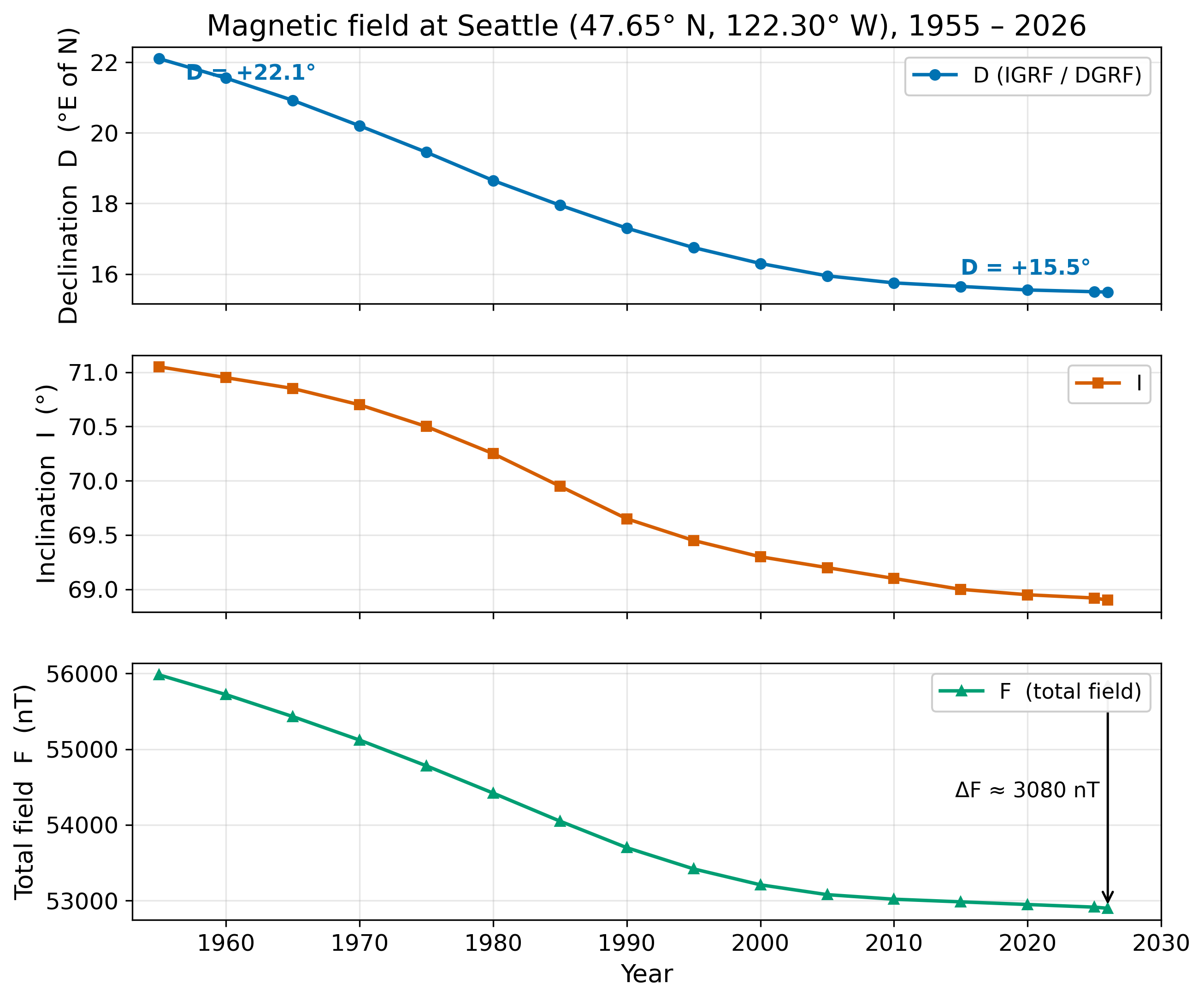— Fig. 106 Secular variation of declination $D$, inclination $I$, and total intensity $F$ at Seattle (47.65° N, 122.30° W) for 1955–2026, derived from the IGRF/DGRF historical models [Alken *et al.*, 2021]. The pace and direction of the drift are reasonably stable on the seven-decade scale but vary appreciably from one decade to the next, occasionally exhibiting an abrupt **geomagnetic jerk** (a rapid change in $\partial \mathbf{B}/\partial t$, on a timescale of months).#

Secular variation has three operational consequences:

Reference epochs. Every magnetic survey is corrected to a reference epoch (the current IGRF epoch) by subtracting the modelled core-field value at the time of observation.
Jerks. Year-scale step changes in the second time derivative of $\mathbf{B}$ — geomagnetic jerks — have been observed in 1969, 1978, 1991, 1999, 2007, 2014, and 2020. Their origin lies in the bulk of the outer core, but their precise hydrodynamic mechanism is debated.
Reversals. Integrated over geological time, secular variation occasionally amounts to a full polarity reversal. The Cretaceous Normal Superchron (118–83 Ma) shows that the reversal rate is not constant; the current rate, $\sim 4$–$5$ reversals per Myr, is among the highest of the Cenozoic. The polarity timescale and its tectonic application are the subject of Lecture 24 §6.

The global dipole moment has declined by about 9% per century since direct measurements began (1840), and the South Atlantic Anomaly — a region over Brazil where the surface field is anomalously weak — has grown by $\sim 1\%$ per year over the satellite era. Whether this declining trend foreshadows a reversal on the geologic timescale (centuries to millennia from now) is an open question; for civil-aviation and satellite-navigation purposes the IGRF is updated every five years to keep the model current.

7. Research horizon — Swarm and the next decade of core science#

The IGRF is built every five years from observatory data and from satellite measurements that map the field globally to spherical-harmonic degrees $n \lesssim 130$ [Alken et al., 2021]. The currently flying constellation is Swarm, three ESA spacecraft launched in 2013 (operating beyond design lifetime). Swarm measures the vector field at $\sim 460$ km altitude with sub-nT precision, which is good enough to:

Track westward drift of the magnetic equator at $\sim 0.2°$ per year — a signature of azimuthal flow at the top of the outer core, consistent with hydrodynamic geodynamo models.
Detect geomagnetic jerks in near-real time and locate their hemispheric source via the rapid change in the third spherical-harmonic time derivative.
Image the lithospheric field at degree $n \sim 130$, exposing oceanic-spreading fabrics, large impact structures (Vredefort, Sudbury), and continental-margin gradient zones.

The geophysical question driving this work — what is happening in the outer core right now? — is central to long-range geomagnetic reference models for civil aviation and satellite navigation, and to ongoing efforts to forecast jerks and reversals. The follow-on mission NanoMagSat (planned 2027) will add a CubeSat constellation for higher-cadence observations.

8. AI literacy — using a language model as a derivation partner#

Equations (178) and (180) are clean enough that a competent large language model (LLM) can be asked to derive them from the vector dipole expression (177). This is a useful test of the model’s mathematical reasoning, and of the student’s ability to check the result.

Reasoning Partner activity

Step 1 — Ask the LLM to derive (178). Prompt: “Starting from the vector form $\mathbf{B}(\mathbf{r}) = (\mu_0/4\pi)(3(\mathbf{m}\cdot\hat{\mathbf{r}})\hat{\mathbf{r}} - \mathbf{m})/r^3$ for a point magnetic dipole, derive the radial and tangential components in spherical polar coordinates aligned with the dipole axis. Show each step.”

Step 2 — Verify, do not trust. Three checks the student must perform:

Does the LLM correctly identify $\mathbf{m}\cdot\hat{\mathbf{r}} = m\cos\theta$ when $\theta$ is the colatitude?
Does the algebra produce the factor-of-2 difference between $B_r$ and $B_\theta$? (A common LLM mistake is to drop the 2 or to misplace it on the $B_\theta$ component.)
Does the final formula use colatitude (angle from the pole) or latitude (angle from the equator)? The two differ by $\pi/2$ and the resulting $\tan I = 2 \tan\lambda$ becomes $\tan I = 2\cot\theta$.

Step 3 — Disagree productively. If the LLM’s derivation has an error, write a one-sentence prompt that identifies the specific step. Do not simply ask “is this right?” — that elicits agreement regardless of the actual answer.

The student deliverable is a one-page record showing: (i) the LLM’s derivation, (ii) at least one identified error or unclear step, and (iii) the corrected derivation in the student’s own notation, signed.

9. Concept check#

Concept-check questions

B versus H in a basalt. A magnetite-bearing basalt has volume susceptibility $\chi \approx 0.05$. If you place it in Earth’s ambient field ($|\mathbf{B}_\text{ext}| = 50\,000$ nT, so $|\mathbf{H}_\text{ext}| = 40\,\text{A m}^{-1}$), what is the induced magnetisation $|\mathbf{M}|$ inside the rock, and by what fraction does $|\mathbf{B}|$ inside the rock exceed the external $|\mathbf{B}_\text{ext}|$?
$(D, I, F)$ at Seattle in 1955. Given the 1955 IGRF values $D = +22.1°$, $I = +71.0°$, $F = 55\,980$ nT, compute the local components $(X, Y, Z)$ at Seattle. Compare with the 2026 values quoted in §3b. Which component has changed the most in relative terms? Which has changed the most in absolute (nT) terms?
Geocentric axial dipole. A paleomagnetic lab measures an inclination of $I = 35° \pm 3°$ on a 50-Myr-old basalt. Use (180) to compute the inferred paleo-latitude and propagate the $1\sigma$ uncertainty. Why is the inversion more reliable at high inclination than at low?
Tangent cylinder. Why do geodynamo simulations consistently put high-latitude flux concentrations just inside the tangent cylinder rather than smoothly distributed over latitude?

Concept-check answers

Answers and worked solutions are provided in the instructor materials (see concept_check_lecture23.md in the ess314-instructor repository).

10. Connections#

Backward to Lecture 22 — Density and the Lithosphere: the same harmonic-attenuation argument that filters the geodynamo field down to its dipole component governs the depth-resolution of gravity surveys (the upward-continuation operator).
Forward to Lecture 24 — Rock Magnetism: the constitutive relation $\mathbf{M} = \chi\mathbf{H}$ of §2 acquires new content when $\chi$ becomes a property of crystal-lattice spin ordering and when rocks can carry a remanent magnetisation $\mathbf{M}_r$ in the absence of any applied field.
Forward to Lecture 25 — Magnetic Anomalies & Surveys: the same dipole expressions (177)–(178) that describe the global field also describe — at the local scale and with $\mu_0\mathbf{m}/(4\pi)$ replaced by $MV/(4\pi)$ — the surface anomaly of a magnetised crustal body.

11. Further reading#

[1] (1,2,3,4)

P. Alken, E. Thébault, C. D. Beggan, H. Amit, J. Aubert, J. Baerenzung, T. N. Bondar, W. J. Brown, S. Califf, A. Chambodut, A. Chulliat, G. A. Cox, C. C. Finlay, A. Fournier, N. Gillet, A. Grayver, M. D. Hammer, M. Holschneider, L. Huder, G. Hulot, T. Jager, C. Kloss, M. Korte, W. Kuang, A. Kuvshinov, B. Langlais, J.-M. Léger, V. Lesur, P. W. Livermore, F. J. Lowes, S. Macmillan, W. Magnes, M. Mandea, S. Marsal, J. Matzka, M. C. Metman, T. Minami, A. Morschhauser, J. E. Mound, M. Nair, S. Nakano, N. Olsen, F. J. Pavon-Carrasco, V. G. Petrov, G. Ropp, M. Rother, T. J. Sabaka, S. Sanchez, D. Saturnino, N. R. Schnepf, X. Shen, C. Stolle, L. Tøffner-Clausen, H. Toh, J. M. Torta, J. Varner, F. Vervelidou, P. Vigneron, I. Wardinski, J. Wicht, A. Woods, Y. Yang, Z. Zeren, and B. Zhou. International geomagnetic reference field: the thirteenth generation. Earth, Planets and Space, 73(1):49, 2021. Open access (CC BY). doi:10.1186/s40623-020-01288-x.

[2]

William Lowrie and Andreas Fichtner. Fundamentals of Geophysics. Cambridge University Press, Cambridge, UK, 3rd edition, 2020. ISBN 978-1108716970. doi:10.1017/9781108685917.

[3]

S. Maus. The geomagnetic power spectrum. Geophysical Journal International, 174(1):135–142, 2008. doi:10.1111/j.1365-246X.2008.03820.x.

Companion notebook (next step)

The accompanying Jupyter notebook magnetics_forward.ipynb (in the notebooks/Lab8/ directory) walks through the IGRF-13 calculator, $(D, I, F) \leftrightarrow (X, Y, Z)$ conversion, and the GAD paleo-latitude inversion with uncertainty propagation.

Open notebook →

Next lecture

L24 — Rock Magnetism builds on the $\mathbf{B}$–$\mathbf{H}$–$\mathbf{M}$ framework introduced today and asks: which minerals carry the lithospheric signal, and how do they record the field?


Course LOs addressed	LO-1 (observables ↔ Earth properties), LO-2 (forward model from source physics to surface field), LO-4 (method strengths, limitations, and uncertainty)
Learning outcomes practiced	LO-OUT-A (predict surface signature from a simple source model), LO-OUT-C (interpret a measurement as a constraint on subsurface structure with appropriate uncertainty)
Prior lecture	L22 — Density and the Lithosphere
Next lecture	L24 — Rock Magnetism
Lab connection	Lab 8 — Magnetic Anomaly Modeling (forward + inverse, induced dipole)
Textbook	Lowrie & Fichtner (2020), Ch. 5.1–5.3; Olson (2015) for the geodynamo

Symbol	Name	Units / notes
\(\mathbf{B}\)	Magnetic flux density — what a magnetometer measures (Lorentz-force field). (L23–L25)	T; nT \(= 10^{-9}\) T
\(\mathbf{H}\)	Auxiliary magnetic field; produced by free currents alone. (L23–L25)	A m\(^{-1}\)
\(\mathbf{M}\)	Magnetisation — volume density of atomic dipole moments. (L23–L25)	A m\(^{-1}\)
\(\mu_0\)	Permeability of free space. (L23–L25)	\(4\pi\times 10^{-7}\) T m A\(^{-1}\)
\(\mu\)	Material permeability: \(\mu = \mu_0(1+\chi)\).	T m A\(^{-1}\)
\(\chi\)	Volume magnetic susceptibility — linear-response coefficient \(\mathbf{M}=\chi\mathbf{H}\). (L23–L25)	dimensionless (SI)
\(F\)	Total field intensity at a station: $F =	\mathbf{B}
\(\mathbf{F}\)	Total-field vector at a station (same magnitude \(F\)).	nT
\(D\)	Declination — horizontal angle of \(\mathbf{F}\) east of true north. (L23–L25)	degrees
\(I\)	Inclination — angle of \(\mathbf{F}\) below horizontal. (L23–L25)	degrees
\(X,\,Y,\,Z\)	Local Cartesian components of \(\mathbf{F}\) (north / east / down).	nT
\(H_\text{horiz}\)	Horizontal magnitude \(H_\text{horiz} = F\cos I\) (subscripted to avoid clash with \(\mathbf{H}\)).	nT
\(\mathbf{m}\)	Magnetic dipole moment — Earth’s geomagnetic moment in L23; a buried-body moment in L25. (L23, L25)	A m\(^2\)
\(r\), \(\hat{\mathbf{r}}\)	Radial distance from the dipole and its unit vector.	m, —
\(\theta\)	Magnetic colatitude (angle from the dipole north pole).	rad / degrees
\(\lambda\)	Geographic latitude (used in \(\tan I = 2\tan\lambda\)). (L23, L24)	degrees
\(B_r,\,B_\theta\)	Radial and tangential components of the dipole field.	nT
\(n\)	Spherical-harmonic degree (Mauersberger–Lowes spectrum).	integer
\(R_n\)	Power per harmonic degree of the surface field.	nT\(^2\)
\(r_\text{CMB},\,r_\text{surf}\)	Core-mantle-boundary and Earth-surface radii (3 480 km; 6 371 km).	km
\(\mathbf{u}\)	Outer-core fluid velocity.	m s\(^{-1}\)
\(\eta\)	Magnetic diffusivity, \(\eta = 1/(\mu_0\sigma)\).	m\(^2\) s\(^{-1}\)
\(\sigma\)	Electrical conductivity of liquid iron (\(\sim 10^6\)).	S m\(^{-1}\)
\(R_m\)	Magnetic Reynolds number, \(R_m = UL/\eta\).	dimensionless
\(Ro\)	Rossby number, \(Ro = U/(2\Omega L)\).	dimensionless
\(\Omega\)	Earth’s rotation rate (\(7.27\times 10^{-5}\) rad s\(^{-1}\)).	rad s\(^{-1}\)
\(T_C\)	Curie temperature (introduced in detail in L24). (L23–L25)	°C