Earth’s Gravity Field and the Geoid

Earth’s Gravity Field and the Geoid#

Prerequisites#

Students should be comfortable with vector calculus at the level of a gradient and a divergence, with Newton’s second law, and with the introductory-physics treatment of central forces. Familiarity with spherical and ellipsoidal coordinates is helpful but not required. The seismology modules established that geophysical methods infer interior structure from surface measurements; gravity is the first non-seismic method that follows the same logic — observation → forward model → inverse problem.

1. The Geoscientific Question#

Two stations sit on the same line of longitude. One is at the foot of Mount Rainier; the other floats on the surface of Puget Sound thirty kilometres to the west. Both gravimeters read out the local value of the acceleration of free fall, \(g\), to a precision of better than one part in a million. The two readings differ by tens of milligals.

Why?

A complete answer requires three pieces. The first is that the Earth is not a point mass — it has a shape, a rotation, and an internal density distribution. The second is that the Mt. Rainier station is at a different elevation, so it is farther from the centre of mass of the Earth, and there is rock between the station and sea level that exerts its own attraction. The third is that the rocks beneath the two stations are not the same: a Quaternary basalt edifice over a sedimentary basin has very different density than the unweathered Cascade arc crust.

Each of these pieces translates a measurable quantity — acceleration — into something a geoscientist actually wants to know: where the mass is, how it is distributed, and how it is changing. The first lecture in the gravity module establishes the framework that makes those translations possible. Fig. 88 already hints at the magnitude of the elevation effect: a few hundred milligals between the surface and low Earth orbit, but only about three milligals between sea level and the summit of Mount Everest. Gravity is exquisitely sensitive over short distances, and numerically tractable over the entire Earth.

Two-panel figure. The left panel plots gravitational acceleration g as a function of normalized radius r / R_E on log-log axes from sea level to ten Earth radii, showing a smooth inverse-square decay; reference points are marked at sea level (~9.82 m/s²), Mt. Everest summit (~9.79 m/s²), the International Space Station orbital altitude (~8.66 m/s²), and geostationary altitude (~0.22 m/s²). The right panel zooms in on the first ten kilometres of elevation, comparing the exact inverse-square curve to the linear free-air approximation of −0.3086 mGal per metre; the Everest summit elevation is annotated at about −2700 mGal of decrement. 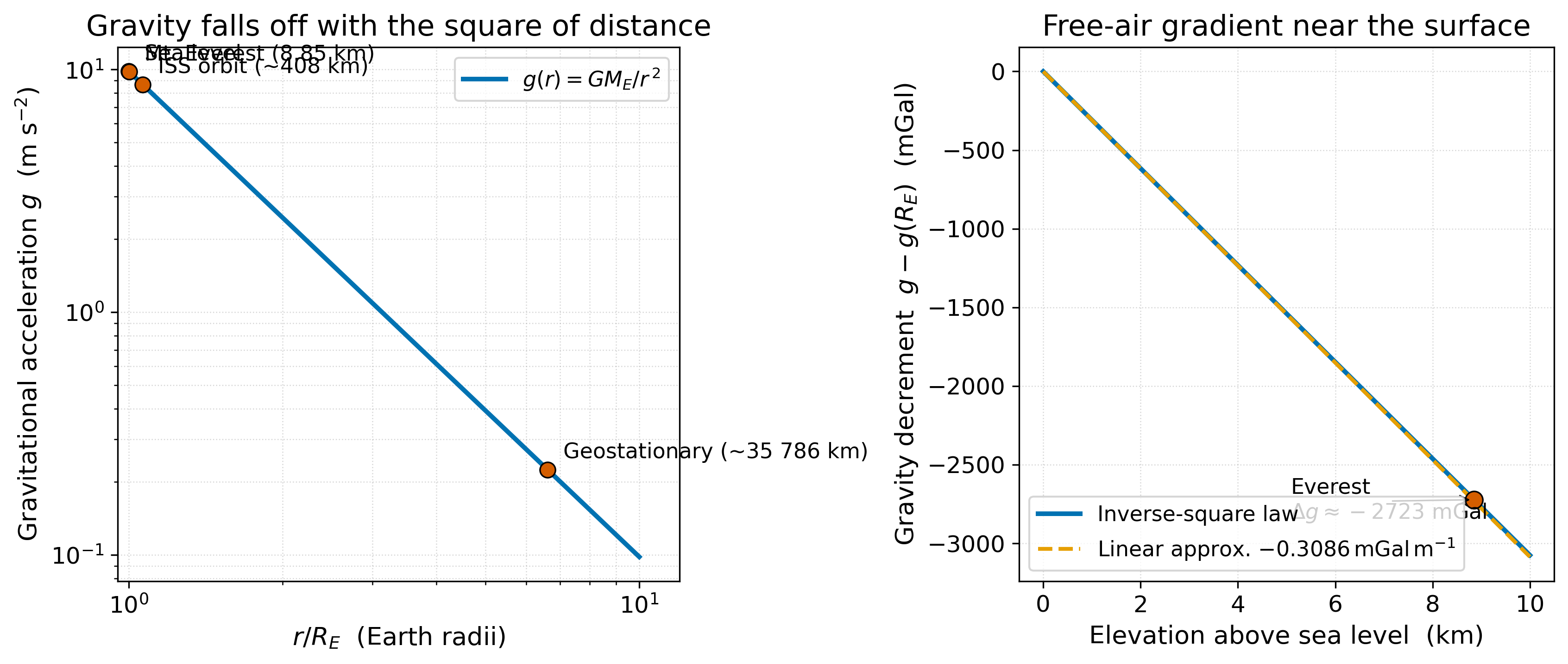— Fig. 88 The inverse-square law of gravitation. Left: \(g\) falls off slowly with distance from Earth’s centre — a useful reminder that ISS astronauts are not weightless because gravity has vanished, but because they are in continuous free fall. Right: near the surface, the linear free-air approximation (\(-0.3086\) mGal per metre) reproduces the inverse-square decay to better than one part in \(10^{4}\) over the full topographic range of Earth.#

2. Governing Physics#

Newton’s law of universal gravitation states that two point masses \(m_{1}\) and \(m_{2}\) separated by a distance \(r\) attract one another along the line joining them with a force whose magnitude is

(144)#\[F = G \, \frac{m_{1} \, m_{2}}{r^{2}}\]

where \(G = 6.67430 \times 10^{-11}\) m³ kg⁻¹ s⁻² is the universal gravitational constant.

Two consequences are worth stating explicitly. First, by Newton’s second law, a unit test mass placed in the gravitational field of a body of mass \(M\) experiences an acceleration of magnitude

(145)#\[g(r) = \frac{F}{m_{\text{test}}} = G \, \frac{M}{r^{\,2}}.\]

The acceleration depends only on the source mass and the distance, not on the test mass. This is why all objects fall at the same rate in vacuum, a fact whose physical meaning escaped Aristotle and was first quantified by Galileo.

Second, the gravitational force is conservative: it can be derived from a scalar potential \(U\) by

(146)#\[\mathbf{g}(\mathbf{r}) = -\nabla U(\mathbf{r}), \qquad U(\mathbf{r}) = -\, G \int_{V} \frac{\rho(\mathbf{r}')}{|\mathbf{r} - \mathbf{r}'|}\, dV',\]

where the integral runs over the Earth’s volume \(V\) and \(\rho(\mathbf{r}')\) is the local mass density. Because \(\mathbf{g}\) is the gradient of a scalar, surfaces of constant \(U\) are everywhere perpendicular to \(\mathbf{g}\). These equipotential surfaces are what is meant by the words “horizontal” and “vertical” — a plumb line points along \(\mathbf{g}\), and a still water surface follows an equipotential. Both definitions ignore the rotation of the Earth, which contributes a centrifugal term that we will fold into the latitude correction in §3.

Key concept — gravity is a field

The acceleration \(\mathbf{g}(\mathbf{r})\) is defined at every point in space, not just at the location of a particular mass. Two consequences follow. First, contributions from different mass elements add linearly: the gravity of the Earth is the integral of contributions from every gram of rock, water, and ice. Second, the geophysical inverse problem — what mass distribution produced the observed field? — is non-unique even in principle. Two different density models can produce identical surface gravity. We will return to this point in Lecture 20.

3. Mathematical Framework#

Notation used throughout this lecture

Symbol	Meaning	Units
\(G\)	Universal gravitational constant	\(6.67430 \times 10^{-11}\) m³ kg⁻¹ s⁻²
\(M_{E}\)	Mass of the Earth	\(5.972 \times 10^{24}\) kg
\(R_{E}\)	Mean Earth radius	\(6.371 \times 10^{6}\) m
\(a\), \(b\)	WGS84 semi-major / semi-minor axes	\(6\,378\,137\) m / \(6\,356\,752\) m
\(f\)	Flattening of the reference ellipsoid	\(1/298.257\) (dimensionless)
\(\varphi\)	Geographic latitude	radians or degrees
\(h\)	Elevation above the reference ellipsoid	m
\(\rho_{c}\)	Average crustal density	typically \(2670\) kg m⁻³
\(g_{n}(\varphi)\)	“Normal” theoretical gravity on the reference ellipsoid	mGal
\(g_{\text{obs}}\)	Measured gravity at the station	mGal
\(\Delta g\)	Gravity anomaly (subscripted by reduction step)	mGal
\(N\)	Geoid undulation (height of geoid above ellipsoid)	m

One milligal (mGal) equals \(10^{-5}\) m s⁻², or about one part in \(10^{6}\) of average surface gravity.

3.1 Three approximations to Earth’s shape#

The simplest model is a uniform sphere. The next is an oblate spheroid — the equilibrium shape of a self-gravitating fluid spinning at the Earth’s angular velocity. The flattest approximation accounting for rotation alone gives a polar radius about 21 km shorter than the equatorial radius. The Earth’s actual flattening, \(f \approx 1/298.257\), is slightly more than this fluid prediction, indicating that the planet’s interior is not a perfect rotating fluid: subtle long-wavelength density variations supported by mantle viscosity perturb the shape.

The third approximation is the geoid itself: the equipotential surface that coincides on average with mean sea level over the oceans. Because mass is unevenly distributed inside the Earth — denser slabs in subduction zones, lighter cratonic roots, oceanic plateaus, ice sheets — the geoid undulates with respect to the reference ellipsoid by amounts ranging from about \(-105\) m near south India to \(+85\) m north of Australia. Fig. 89 summarises the hierarchy.

Three side-by-side panels comparing concentric profiles of the Earth. Panel (a) shows a perfect sphere with a small cross marking the centre. Panel (b) shows an oblate spheroid with the equatorial sphere drawn as a dotted reference circle and a red arrow indicating polar flattening; the flattening is exaggerated 100-fold for visibility. Panel (c) shows the geoid as a green deviation from the dashed reference-ellipsoid contour, with characteristic large-amplitude undulations exaggerated 8000-fold so the lumpy shape is visible. 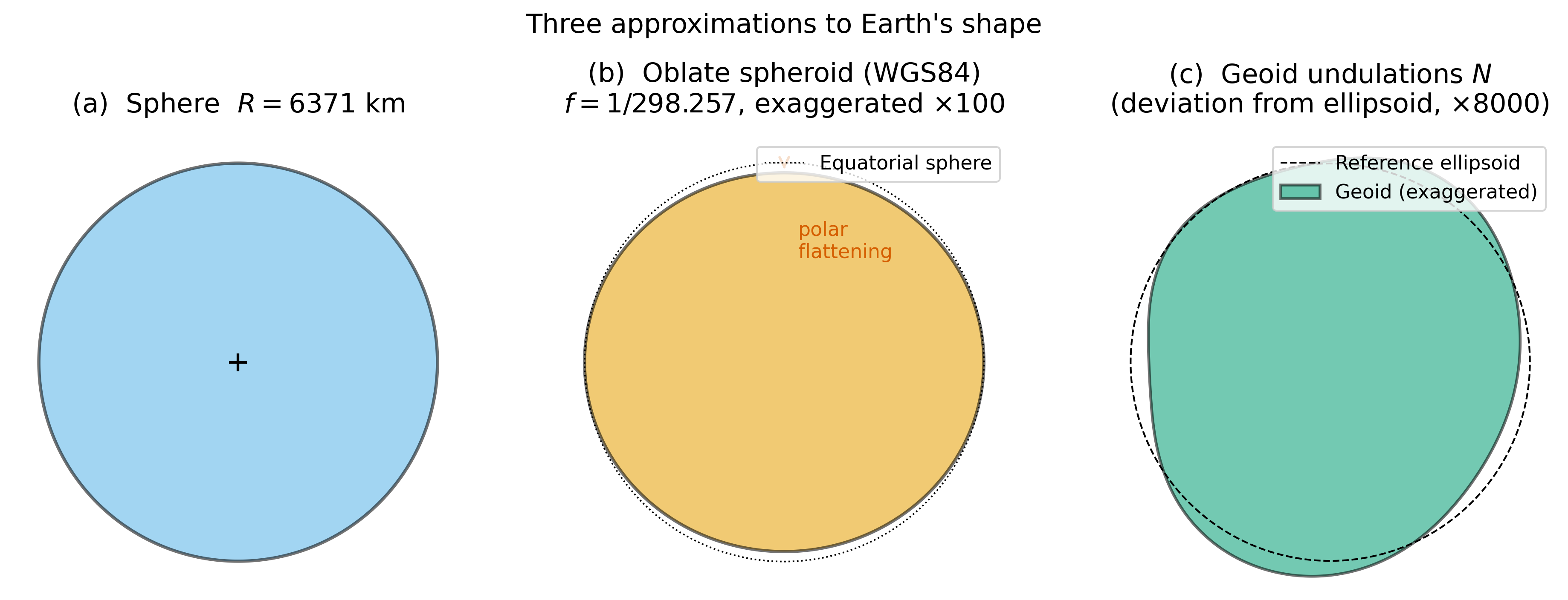— Fig. 89 Three successive approximations to Earth’s shape. (a) The sphere of mean radius reproduces gravity to a few parts in a thousand. (b) The reference ellipsoid (WGS84) accounts for rotation and is the basis of latitude-corrected “normal” gravity. (c) The geoid — drawn here at 8000× exaggeration — is the equipotential surface used for measuring elevation; ocean tide gauges sit on it within centimetres.#

3.2 Theoretical gravity at the reference ellipsoid#

The theoretical gravity \(g_{n}(\varphi)\) on the GRS80 reference ellipsoid is, to good approximation,

(147)#\[g_{n}(\varphi) \approx 978\,032.7 \, \bigl( 1 + 0.00530245 \sin^{2}\varphi - 0.00000582 \sin^{2}2\varphi \bigr) \;\;\text{mGal}.\]

This formula combines the inverse-square contribution of the Earth’s mass distribution, the centrifugal term from rotation, and the second-order correction for the ellipsoidal shape. At the equator \(g_{n} \approx 978\,033\) mGal; at the poles \(g_{n} \approx 983\,219\) mGal. The total equator-to-pole difference is about \(5\,186\) mGal, dominated almost entirely by rotation: the centrifugal acceleration at the equator is \(\omega^{2} R \approx 3\,375\) mGal directed outward, plus the equatorial bulge moves the surface farther from the centre and so reduces \(g\) by an additional \(1\,800\) mGal or so.

3.3 Why is Earth’s gravity measured to four extra decimal places?#

A gravimeter measures \(g\) to about \(\pm 0.01\) mGal, or one part in \(10^{8}\) of \(g\). Targets of geophysical interest produce signals of order \(0.1\)–\(100\) mGal, so the precision is not gratuitous. Fig. 90 traces the budget for a synthetic 200-km transect over a mountain range, a valley, and a buried high-density body. The raw deviation from normal gravity is dominated by elevation effects (\(\sim 300\) mGal); the buried body’s signature, which is the actual geological target, is only about 5 mGal and emerges only after the four corrections described below have been applied.

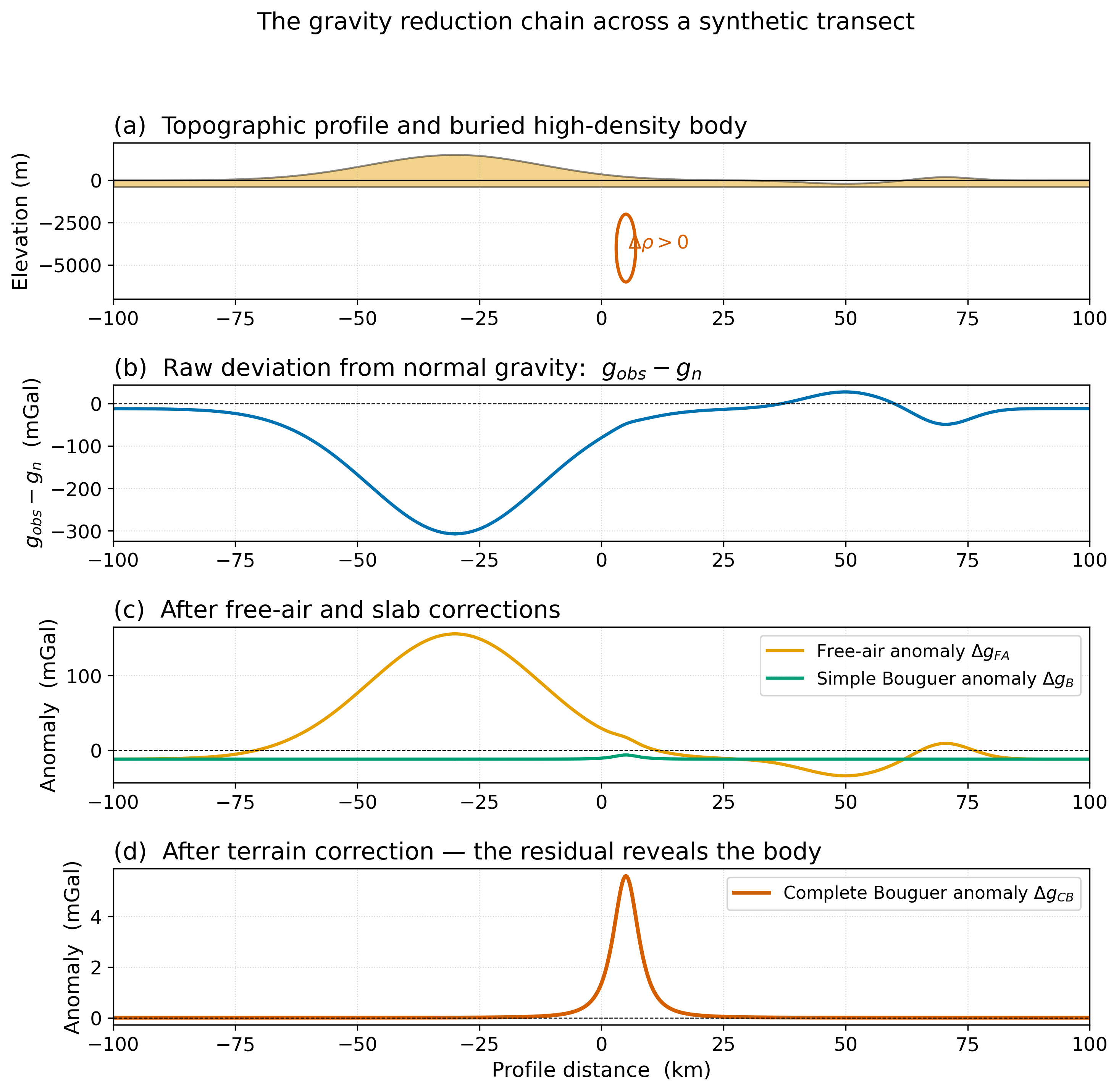
Fig. 90 The gravity reduction chain. The buried density anomaly that motivated the survey produces only 5 mGal of signal, against an elevation-driven background of 300 mGal. Each correction below is designed to remove a specific, predictable contribution.#

3.4 The four corrections#

Latitude correction. The “normal” gravity of equation (147) is subtracted from the observation:

(148)#\[\Delta g_{\text{raw}} = g_{\text{obs}} - g_{n}(\varphi).\]

This removes the effect of Earth’s rotation and ellipticity.

Free-air correction. A station at elevation \(h\) above the reference ellipsoid is farther from Earth’s centre, so \(g\) is smaller there. Differentiating equation (145):

(149)#\[\frac{dg}{dr} = -2\,\frac{G M_{E}}{r^{3}} = -\frac{2 g}{r}.\]

Evaluated at \(r = R_{E}\) this gives \(-0.3086\) mGal per metre. The free-air correction added to the observation is therefore

(150)#\[\text{FA}_{\text{corr}} = +\,0.3086 \, h \;\;\text{(mGal, with } h \text{ in m)}.\]

The free-air anomaly is

(151)#\[\Delta g_{\text{FA}} = g_{\text{obs}} - g_{n}(\varphi) + \text{FA}_{\text{corr}}.\]

Bouguer (slab) correction. A station at elevation \(h\) has rock between it and sea level, and that rock pulls the gravimeter down — a positive contribution to the measurement. Approximating the rock between the station and sea level as an infinite horizontal slab of density \(\rho_{c}\) and thickness \(h\), an exercise in cylindrical symmetry yields

(152)#\[g_{\text{slab}} = 2\pi G \rho_{c} h.\]

In milligals, with \(\rho_{c}\) in g cm⁻³ and \(h\) in metres, the Bouguer correction is

(153)#\[\text{B}_{\text{corr}} = -\,0.0419 \times 10^{-3} \, \rho_{c} \, h \;\;\text{(mGal)}.\]

For the standard reduction density \(\rho_{c} = 2.67\) g cm⁻³ this is \(-0.112\) mGal m⁻¹, partially cancelling the free-air correction. The combined elevation correction is the net free-air-plus-Bouguer slope, \(0.197\) mGal per metre of elevation for normal-density crust.

Terrain correction. A real survey is not over a flat plateau. Mountains above the station pull the gravimeter laterally and slightly upward, reducing \(g\); valleys below the station leave a mass deficit relative to the assumed Bouguer slab. The terrain correction is always positive — it is added to the simple Bouguer anomaly to give the complete Bouguer anomaly:

(154)#\[\Delta g_{\text{CB}} = g_{\text{obs}} - g_{n}(\varphi) + \text{FA}_{\text{corr}} - \text{B}_{\text{corr}} + \text{T}_{\text{corr}}.\]

In rugged terrain (Cascades, Andes), the terrain correction can exceed 10 mGal. Modern processing computes it numerically from a digital elevation model; classical hand processing used the Hammer chart, a cylindrical grid invented at the University of Washington in 1939.

Key equation — the complete reduction

The complete Bouguer anomaly is what gravity surveyors actually report:

\[ \Delta g_{\text{CB}}\;=\;g_{\text{obs}}\;-\;g_{n}(\varphi)\;+\;0.3086\,h\;-\;0.0419\!\times\!10^{-3}\rho_{c}\,h\;+\;\text{T}_{\text{corr}}\;. \]

Whatever signal remains is, by construction, due to lateral density variations beneath the survey — the actual geological target.

4. The Forward Problem#

Given a model of the Earth — its shape, its density distribution, the topography between the station and the geoid — one can predict the gravity that a station should measure. The forward problem in §3 has two parts. The first is the spheroidal reference field \(g_{n}(\varphi)\), which captures everything about the Earth’s bulk shape and rotation. The second is the deviation from \(g_{n}\) produced by topography and lateral density variations near the surface, which is the engine of equation (154).

A well-posed forward calculation requires three inputs: latitude, elevation, and a density model for the rock above the geoid. Surveyors choose the reduction density \(\rho_{c}\) to minimise the correlation between the resulting Bouguer anomaly and topography. For “normal” crust, \(\rho_{c} = 2.67\) g cm⁻³. For the basalt-veneer of an oceanic plateau, \(\rho_{c}\) is closer to \(2.95\) g cm⁻³. Choosing the wrong reduction density introduces a topography-correlated artifact that masquerades as a real anomaly — a useful diagnostic in its own right.

The companion notebook gravity_corrections.ipynb implements the full reduction chain on a synthetic transect. Students choose station locations along a digital elevation model, set a reduction density, and observe how each correction unmasks the embedded subsurface anomaly.

5. The Inverse Problem#

The inverse problem in this lecture is mostly a bookkeeping inverse problem rather than a geophysical one. Given the measured \(g_{\text{obs}}\), latitude, elevation, and topography, equation (154) recovers the residual signal \(\Delta g_{\text{CB}}\). This residual is what feeds the more interesting inverse problem of Lecture 20: given an observed anomaly, what subsurface mass distribution produced it?

Two non-uniqueness statements anchor the conversation that follows. First, gravity is an integral of \(\rho(\mathbf{r}')\) — many density models produce the same surface anomaly, so depth and density-contrast are formally inseparable. Second, an unknown error in the reduction density introduces a topography-correlated artifact in \(\Delta g_{\text{CB}}\) that is not distinguishable from a real anomaly correlated with elevation. Both statements point to the same epistemic reality: gravity alone is rarely enough. Combining gravity with seismic constraints on density structure or with magnetic constraints on lithology is the rule, not the exception, in published interpretations.

6. Worked Example — Three Numbers Every Geophysicist Should Carry#

Estimate the four corrections for a station at \(\varphi = 45^{\circ}\) N, elevation \(h = 2000\) m, with surrounding terrain rising another \(300\) m on average within 5 km of the station.

Latitude correction. From equation (147),

\[ g_{n}(45^{\circ}) = 978\,032.7 \, (1 + 0.00530245 \cdot 0.5 - 0.00000582 \cdot 1.0) \approx 980\,629\;\text{mGal}. \]

Free-air correction. \(0.3086 \times 2000 = 617\) mGal added back to the observation.

Bouguer correction. Using \(\rho_{c} = 2.67\) g cm⁻³,

\[ \text{B}_{\text{corr}} = -\,0.0419 \times 10^{-3} \times 2.67 \times 2000 \approx -224\;\text{mGal}. \]

The combined elevation correction is \(617 - 224 = 393\) mGal — about \(0.197\) mGal per metre of elevation, as expected.

Terrain correction. A rough estimate from the Hammer chart for the geometry given is of order \(+10\) mGal.

The combined correction applied to a raw measurement \(g_{\text{obs}}\) in the alpine setting is therefore \(\approx +400\) mGal. A 5-mGal target — a real geological anomaly — sits two orders of magnitude below the corrections, which is why precision and consistency in the reduction chain matter so much.

Concept check

An observer reports a free-air anomaly of \(+200\) mGal at a 3000-m alpine station. The simple Bouguer anomaly at the same station is \(-150\) mGal. Without doing arithmetic, what does this difference tell you about whether the mountain is locally compensated by a low-density root?
A bathymetric chart shows a 4-km-deep ocean trench. Sketch qualitatively the free-air and simple Bouguer anomalies you would expect across the trench, given that the seawater above the seafloor has density \(\sim 1.03\) g cm⁻³ and the assumed reduction density is \(2.67\) g cm⁻³.
Two stations sit at the same elevation and latitude on opposite sides of a vertical fault. Their Bouguer anomalies differ by \(5\) mGal. Without seismic information, can the data alone tell you the throw on the fault? What additional measurement would constrain the answer?

7. Course Connections#

Backward to seismology (Lectures 11–12, Whole Earth Imaging and Seismic Tomography). Density and seismic velocity are linearly related to first order via empirical scaling laws; combining gravity with tomography sharpens both.
Backward to Module 4 (Earthquakes). The Seattle Fault Zone’s surface trace was recognised in 1992 partly from a sharp gradient in the isostatic-residual gravity field — a topic developed in Lecture 20.
Forward to Lecture 20, where Bouguer-residual anomalies become the input to subsurface-imaging forward and inverse models.
Forward to Lecture 21, where the two large-scale corrections of this lecture are reinterpreted as evidence for isostatic compensation: Earth’s lithosphere systematically supports topography by either thickness variations (Airy) or density variations (Pratt).

8. Research Horizon#

Three open-access threads connect this lecture to current research.

The GRACE-FO mission (NASA / GFZ), launched in 2018, measures the time-varying global gravity field by tracking the separation between two co-orbiting satellites to the precision of a fraction of a micrometre. The mission is the primary instrument for measuring ice-sheet mass loss in Greenland and Antarctica, terrestrial water storage anomalies, and post-seismic deformation of large megathrust earthquakes. For a recent open-access summary of the mission’s contribution to climate science, see Tapley et al. (2019, Nature Climate Change 9, 358–369; https://doi.org/10.1038/s41558-019-0456-2).

A 2023 review by Pail et al. in Surveys in Geophysics (open access, https://doi.org/10.1007/s10712-023-09765-0 (⚠ DOI returns 404 — verify manually)) synthesises the present state of static gravity-field modelling from satellite, airborne, and terrestrial data, and identifies the centimetre-level geoid as a near-term goal.

A 2024 paper by Cleves et al. (Geophysical Research Letters, open access via author manuscript) demonstrates that gravity-anomaly time series can resolve the migration of fluid pulses associated with slow-slip events along the Cascadia subduction zone. The result connects gravity directly to the subduction-zone earthquake-cycle problem covered in Lecture 18.

9. Societal Relevance — The Earth is Losing Mass#

In 2002, GRACE began measuring a steady, broad gravity decrease over Greenland. The signal, after correction for ocean tides and continental hydrology, corresponds to about \(270\) Gt yr⁻¹ of ice mass loss, accelerating roughly linearly through the mission lifetime. GRACE-FO, the follow-on mission, has continued the measurement since 2018 and shows that the rate is now substantially higher.

For the Pacific Northwest, two consequences follow. First, the centre-of-mass shift of the global cryosphere alters the orientation of the geoid by millimetres at decadal scales — a measurable signal in regional sea-level change that complicates tide-gauge interpretation around Puget Sound. Second, regional gravity changes from groundwater extraction, especially in the Columbia Plateau aquifer system, are within an order of magnitude of being detectable by next-generation airborne gravity surveys. A useful follow-up is the USGS report “Groundwater Storage Changes in the Columbia Plateau Regional Aquifer System” (Burns et al., USGS SIR 2010-5101, public domain).

AI Literacy — AI as a Tool#

Modern processing of satellite gravity data uses machine learning at two stages. The first is gravity-gradient feature extraction from satellite data such as GOCE: convolutional neural networks identify edges and lineaments in the gravity gradient tensor that correspond to faults, basement contacts, and intrusions. The second is neural ensemble inversion: instead of one inversion that produces a single density model, an ensemble of trained neural networks produces a distribution of plausible models that captures the non-uniqueness explicitly.

Both applications illustrate a useful general principle. Machine learning excels at recognising the patterns in a forward map (geology → gravity) that an analyst would otherwise spend hours digitising by eye. It does not solve the underlying physical inverse problem — the non-uniqueness of equation (146) is mathematical, not algorithmic, and no amount of training data removes it. A neural network that is asked “where is the fault?” can be answered confidently. A neural network that is asked “what is the density contrast?” is reporting a posterior, and the posterior must be reported with the same care as any other inverse-problem result.

For an open-access entry point, see Yu et al. (2024), Earth-Science Reviews 248, 104653 — “Deep learning in geophysical inversion: a review of methods and applications” — https://doi.org/10.1016/j.earscirev.2023.104653.


Course LOs addressed	LO-1 (observables ↔ Earth properties), LO-2 (forward model), LO-4 (method strengths and limitations)
Learning outcomes practiced	LO-OUT-A (predict effect of structure), LO-OUT-B (compute first-order responses), LO-OUT-C (explain why a method works)
Prior lecture	L18 — Tsunami
Next lecture	L20 — Gravity Anomalies and Subsurface Modeling
Lab connection	Lab 5 — Gravity Surveys (forward modeling and corrections in Python)
Discussion	Session 5 — Gravity, Ice Sheets, and CO₂