Building Earth Images: The Iterative Refraction–Reflection Workflow

Building Earth Images: The Iterative Refraction–Reflection Workflow#

Prerequisites#

Students should be comfortable with: ray geometry and Snell’s law (Lecture 5); refraction head waves, the intercept-time equation, and first-arrival tomography (Lectures 6–7); normal moveout, CMP stacking, the Dix equation, the hyperbolic travel-time curve $t(x)^2 = t_0^2 + x^2/V_{\rm rms}^2$, and AVO (Lectures 8–9).

1 — The Geoscientific Question#

Off the eastern coast of New Zealand’s North Island, the Pacific plate slides obliquely westward beneath the Australian plate at the Hikurangi subduction zone. The plate interface spans depths from less than 5 km beneath the trench to roughly 20–25 km under the forearc — and its geometry, coupling state, and fluid content control both the size of future megathrust earthquakes and the tsunami hazard to New Zealand’s most populated coastlines.

No borehole reaches this interface. Every constraint on its position, dip, and physical properties comes from seismic imaging. At Hikurangi, modern campaigns deploy ocean-bottom seismometers (OBS) at long offsets to record first-arrival refractions, and a towed hydrophone streamer at shorter offsets to record reflections. Both instrument systems record the same airgun shots — yet they produce complementary datasets that constrain different aspects of the subsurface.

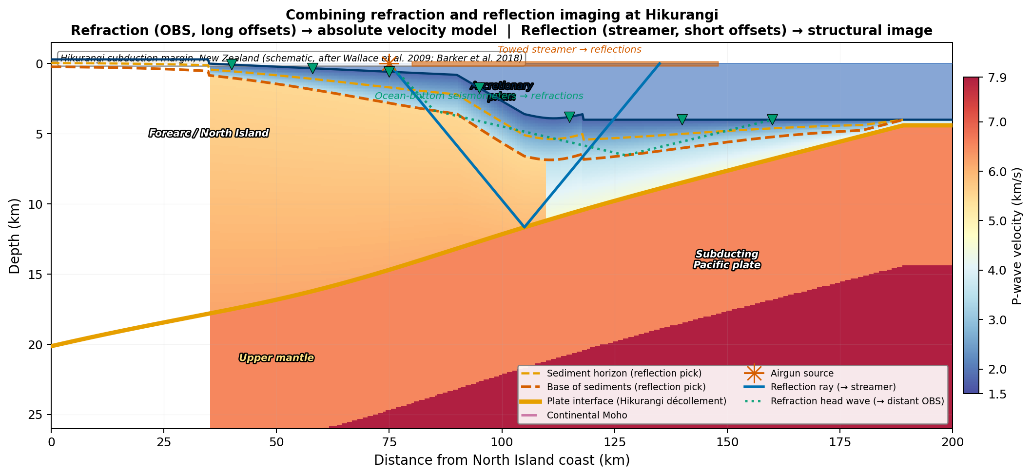
Schematic cross-section of the Hikurangi subduction margin showing the velocity background from refraction (colour) and structural picks from reflection (bold lines), with OBS receivers on the seafloor and a streamer at the sea surface. — Fig. 37 **The Hikurangi subduction margin (schematic after Wallace *et al.* [2009]; Barker *et al.* [2018]).** The background colour shows the P-wave velocity model from wide-angle refraction: slow sediments (blue) grading to fast crust and mantle (orange–red). Dashed lines are reflection picks at key sediment interfaces; the bold yellow–orange line traces the plate interface (décollement). Green triangles mark OBS positions; the dotted green line is a refraction head-wave ray path. The blue solid line is a reflection ray from the airgun to the plate interface and back to the towed streamer. Refraction and reflection are not competing experiments — they are complementary constraints on the same Earth model $v(x,z)$.#

The key insight motivating this lecture is that refraction and reflection are not competing methods — they are two windows onto the same Earth model $v(x,z)$, and combining them iteratively produces better images than either alone. This lecture builds that iterative framework from first principles, starting with the simplest possible case and progressively adding physical complexity.

2 — The Framework: Forward and Inverse Modeling#

2.1 The forward model#

A forward model answers the question: given that I know the Earth model, what data should I expect to record?

In seismic imaging the Earth model $\mathbf{m}$ encodes the velocity field $v(x,z)$ and the reflectivity $r(x,z)$. The forward operator $F$ maps from model space to data space:

(88)#\[\mathbf{d} = F\,\mathbf{m},\]

where $\mathbf{d}$ is the predicted seismic record (time traces at all receivers). In the simplest zero-offset case, $F$ reduces to the kinematic calculation $t = 2z/v$: if a flat reflector sits at depth $z$ in a medium with velocity $v$, the forward model predicts an arrival at two-way time $t = 2z/v$.

Running the forward model is computationally cheap given a model, because it follows the laws of physics directly. It is also the source of all training data for machine-learning surrogates — a point we return to in Section 6.

2.2 The inverse model#

An inverse model answers the question: given the data I recorded, what Earth model produced them?

In principle, invert (210) for $\mathbf{m}$: $$\mathbf{m} = F^{-1}\,\mathbf{d}.$$

In practice, $F^{-1}$ is rarely available: the system is underdetermined, data are noisy, and the operator is nonlinear when the velocity is unknown. The practical strategy uses the adjoint (mathematical transpose) of $F$:

(89)#\[\hat{\mathbf{m}} = F^\top\,\mathbf{d}.\]

The adjoint operator $F^\top$ is called migration. It is not the true inverse, but for a well-sampled survey with a correct velocity model it produces a good approximation of the true reflectivity. The quality of that approximation depends on whether the velocity model is correct — and that is exactly why refraction and reflection imaging must be combined.

Forward vs. inverse — at a glance

	Forward model	Inverse / adjoint (migration)
Question	Given $\mathbf{m}$, predict $\mathbf{d}$	Given $\mathbf{d}$, estimate $\mathbf{m}$
Operator	$F$	$F^\top$
Example	$t = 2z/v$, ray tracing, wave equation	Kirchhoff sum, reverse-time migration
Requires	Earth model + velocity $v$	Observed data + velocity $v$
Output	Synthetic seismogram	Depth image (reflectivity)

Both forward modeling and migration depend on $v(x,z)$. Neither can produce a correct result without it.

3 — Building the Image: From Flat Layers to Full Complexity#

3.1 Case 1 — Single flat layer, constant velocity#

The simplest forward model: one flat reflector at depth $z$, constant velocity $v$. The round-trip time is $t = 2z/v$. The inverse (migration) is exact:

\[z = \frac{v\,t}{2}.\]

Migration here is nothing more than multiplying the two-way time by $v/2$. No horizontal shift is needed, and if the velocity is known, the depth is exact. This is why introductory courses can discuss reflector depths without mentioning migration: for flat layers in a constant-velocity medium, the display is already correct.

3.2 Case 2 — Multiple flat layers: why the velocity model matters#

Real crust has multiple layers with different velocities. For three layers with interval velocities $v_1 < v_2 < v_3$ and interface depths $z_1 < z_2 < z_3$, the zero-offset reflections arrive at:

(90)#\[t_1 = \frac{2z_1}{v_1}, \quad t_2 = t_1 + \frac{2(z_2 - z_1)}{v_2}, \quad t_3 = t_2 + \frac{2(z_3 - z_2)}{v_3}.\]

Converting back from time to depth requires knowing each $v_i$. The Dix equation (Lecture 8) does this from NMO stacking velocities $V_{{\rm rms},n}$:

(91)#\[v_n^2 = \frac{V_{{\rm rms},n}^2\,t_n - V_{{\rm rms},n-1}^2\,t_{n-1}}{t_n - t_{n-1}}.\]

The Dix inversion integrates downward from the surface. Any error in $v_1$ propagates into $v_2$, and both errors propagate into $v_3$. This is where refraction data are indispensable: head-wave analysis (Lectures 6–7) measures absolute interval velocities $v_1, v_2, \ldots$ in the shallow layers, pinning the top of the Dix chain to a known, absolute value.

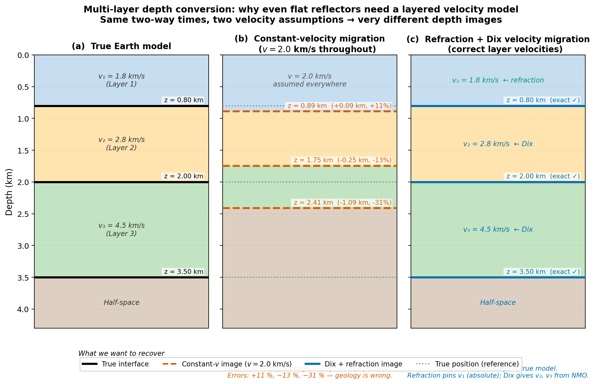
Three panels. Left: true Earth with three horizontal layers at 0.80, 2.00, and 3.50 km with velocities 1.8, 2.8, and 4.5 km/s. Centre: depth image with constant 2.0 km/s, showing errors of plus 11 percent, minus 13 percent, and minus 31 percent. Right: depth image with correct refraction-plus-Dix velocities, with all interfaces at exact depths. — Fig. 38 **Multi-layer depth conversion: same two-way times, two velocity strategies, very different images.** Assuming a constant $v = 2.0$ km/s (centre) places the shallowest reflector 11 % too deep and the deepest 31 % too shallow. Using refraction-derived $v_1$ and Dix-inverted $v_2, v_3$ (right) recovers all three interfaces exactly. The message: even perfectly flat reflectors require the correct layered velocity model.#

Key takeaway — flat reflectors still need a velocity model

The depth error in the deepest reflector is 31 % when a constant velocity is assumed. Refraction provides the near-surface absolute velocity that anchors the Dix inversion; without it, errors at the top of the section corrupt every deeper interval estimate.

3.3 Case 3 — Dipping layers: migration corrects mispositioning#

When a reflector dips at angle $\theta$, a zero-offset recording places events in the wrong lateral and vertical position. The physical reason: the law of reflection requires the ray to hit the reflector at 90° (the normal ray). For a dip $\theta$, the normal ray is not vertical — it travels at $\theta$ off-vertical, reaching the true reflection point $R$ updip and shallower than the point $C$ conventionally plotted directly below $S$.

The two errors are:

\[ \Delta x = d\sin\theta \quad (\text{horizontal: plotted too far downdip}); \qquad \tau = t\cos\theta \quad (\text{corrected two-way time, shorter than recorded } t). \]

Both vanish when $\theta = 0$ (Case 1). Reading the local slope $p_0 = \partial t / \partial y$ from the unmigrated section and using $\sin\theta = vp_0/2$ (Snell’s parameter with the two-way factor), the hand-migration formulas are:

(92)#\[\Delta x = \frac{v^2 p_0 t}{4}, \qquad \tau = t\sqrt{1 - \frac{v^2 p_0^2}{4}}.\]

These corrections again depend on $v$ — reinforcing that migration always requires an accurate velocity model (Cases 1–3 all converge on this point).

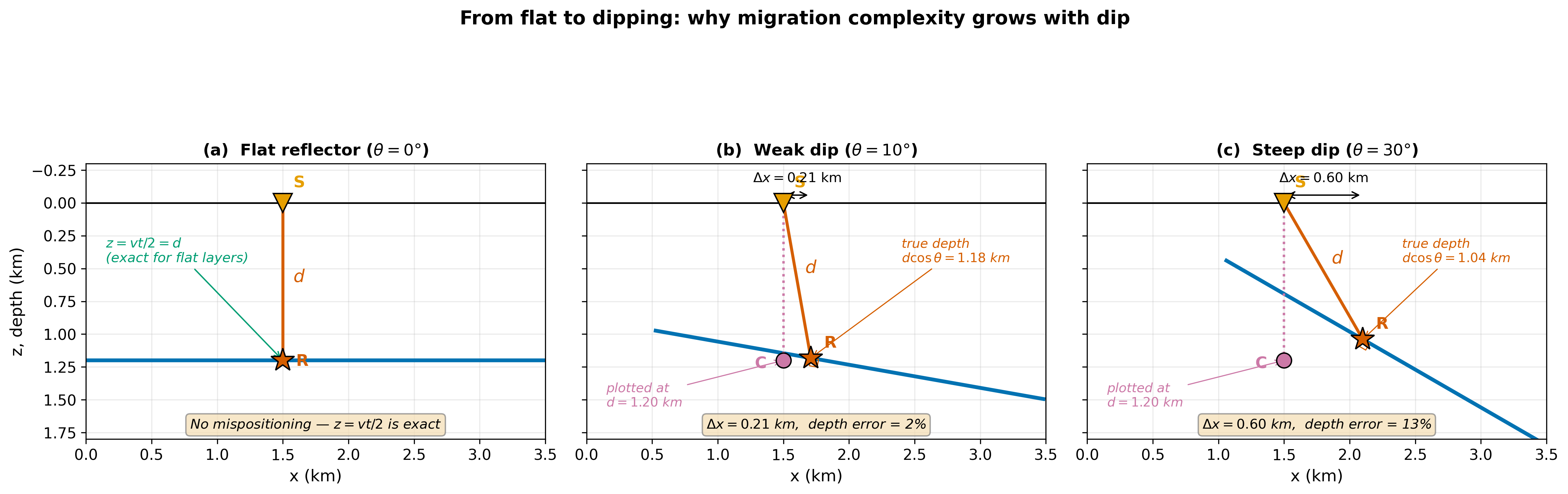
Three panels showing flat (theta=0), weak-dip (theta=10 degrees), and steep-dip (theta=30 degrees) reflectors with the normal ray and apparent vs true positions. — Fig. 39 **From flat to dipping.** At $\theta = 0°$ migration is exact with $z = vt/2$. At $10°$, horizontal and depth errors are small. At $30°$ they are large enough to distort the geological interpretation ($\Delta x = 0.60$ km, 13% depth error). Migration applies (92) to correct both.#

3.4 Case 4 — Diffractions and scatterers: Kirchhoff migration#

Real Earth cross-sections contain fault tips, unconformity edges, rugose basement, and salt flanks — any geometric discontinuity radiates energy as a point diffractor (Huygens’ principle). In a zero-offset time section, a scatterer at $(x_0, z_0)$ produces a diffraction hyperbola:

(93)#\[t(y) = \sqrt{\left(\frac{2z_0}{v}\right)^2 + \left(\frac{2(y - x_0)}{v}\right)^2},\]

with apex directly above the scatterer. An unprocessed section from a structurally complex area is littered with overlapping hyperbolas, as seen in Fig. 40.

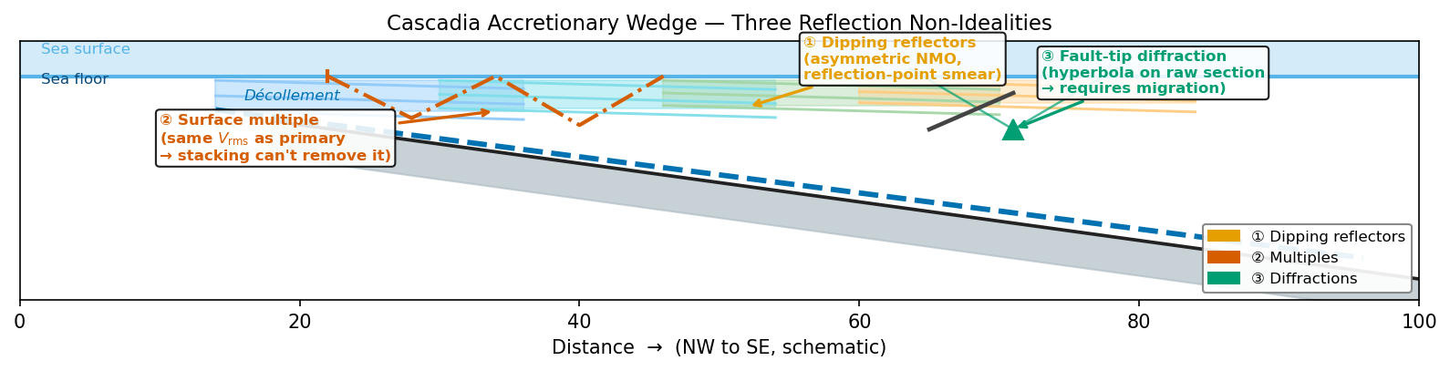
Schematic of the Cascadia accretionary wedge showing dipping reflectors, surface multiples, and a fault-tip diffraction hyperbola. — Fig. 40 **Three challenges in a real accretionary wedge.** (1) Dipping reflectors (Case 3, mispositioning). (2) Surface multiples — same $V_{\rm rms}$ as primary reflections, cannot be removed by NMO stacking alone. (3) A fault-tip diffraction — the raw section shows a hyperbola; migration collapses it to the fault tip.#

Kirchhoff migration collapses each diffraction hyperbola to its source point by summing data along the exact hyperbola (93) and depositing the sum at $(x_0, z_0)$. The forward and adjoint form a dual pair illustrated in Fig. 41:

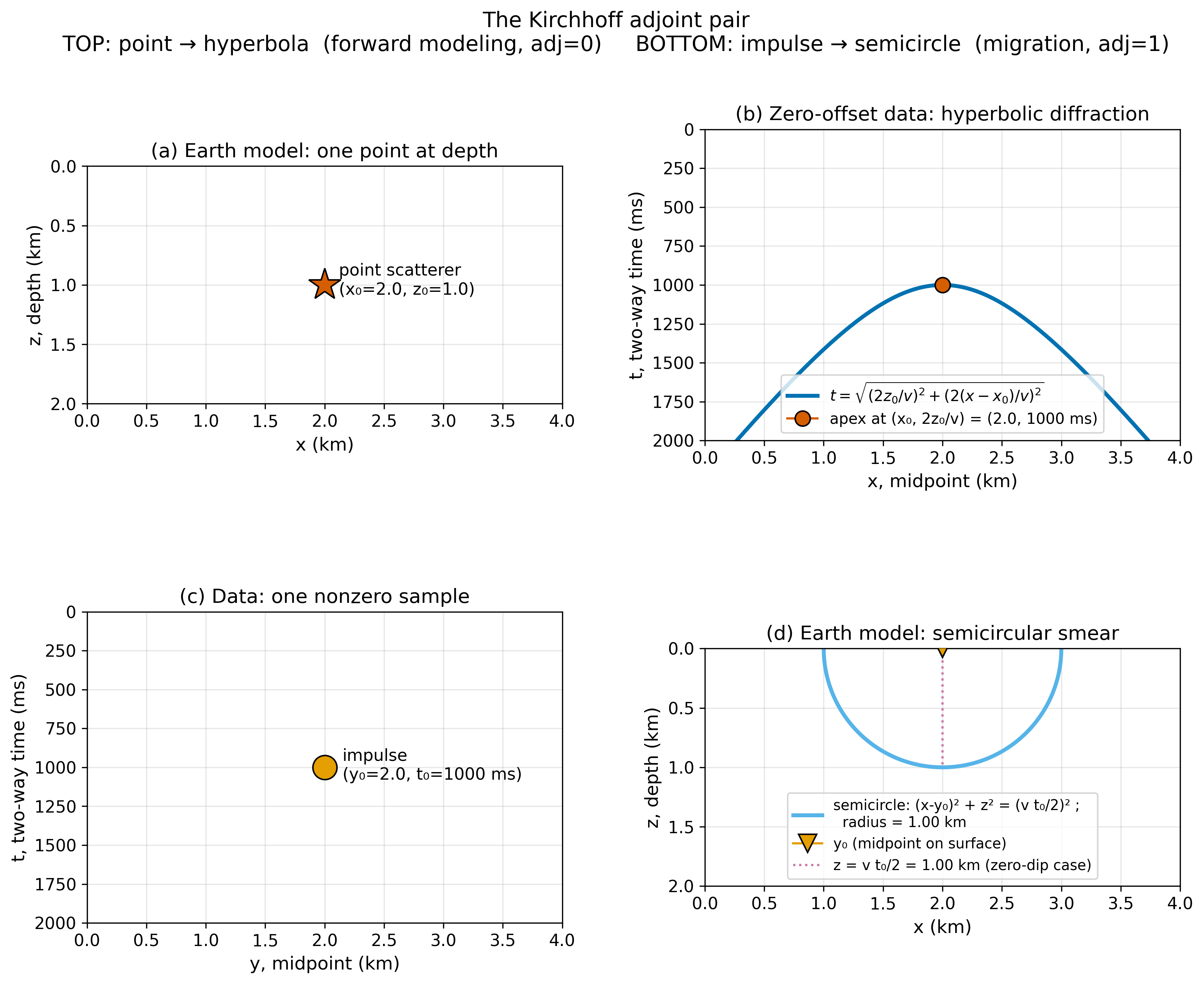
Four panels. Top: forward modeling spreads a point scatterer into a hyperbola. Bottom: migration sums data along the hyperbola to image the point. — Fig. 41 **Kirchhoff adjoint pair.** Forward modeling (top): a point scatterer $\to$ hyperbola in data space. Migration (bottom): data impulse $\to$ semicircle of possible scatterers in model space. Summing all such semicircles for the full dataset collapses each hyperbola back to its source. (Claerbout [2010], subroutine `kirchslow`.)#

In pseudocode, forward modeling and migration share one loop; the only difference is the direction of the copy:

for every (ix, iz) in the model:
    for every midpoint y in the data:
        t = sqrt( (2·z[iz]/v)² + (2·(x[ix]−y)/v)² )    # same hyperbola
        if forward:   data[t, y]    += model[iz, ix]     # spreads scatterer
        else:         model[iz, ix] += data[t, y]        # collapses hyperbola

This is what it means for migration to be the adjoint $F^\top$ of the forward operator $F$: same kinematic geometry, copy direction reversed.

4 — The Velocity–Image Duality#

The Kirchhoff summation in (89) depends explicitly on $v$: the shape of the summation hyperbola is determined by the migration velocity. Using the wrong $v$ produces characteristic geometric residuals — the velocity–image duality — that serve as the primary quality-control signal in the iterative workflow.

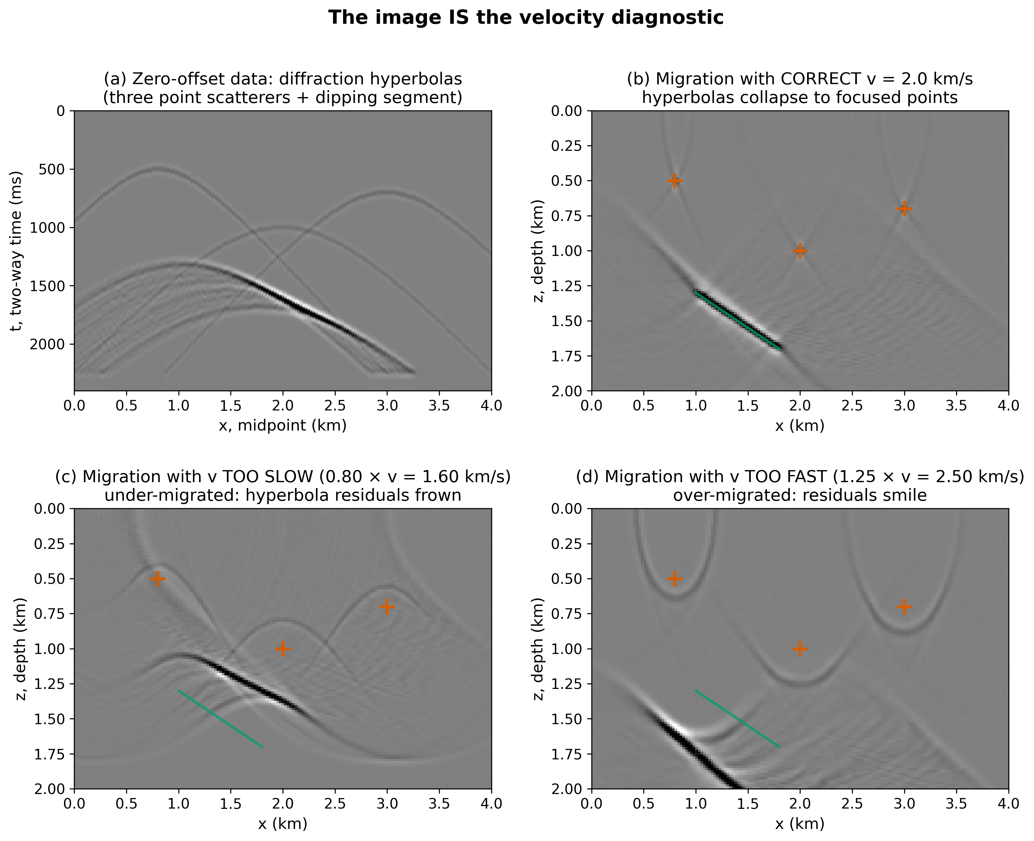
Four panels. Top-left: raw zero-offset data with diffraction hyperbolas. Top-right: correct-velocity migration with focused points. Bottom-left: slow-velocity migration with downward frowns. Bottom-right: fast-velocity migration with upward smiles. — Fig. 42 **The velocity–image duality.** Same data, three migration velocities. Correct $v$ (top right): diffractions collapse to points, reflectors at true positions. Too slow (bottom left): residual downward arcs (“frowns”) — the migration hyperbola is too narrow, leaving flanks behind. Too fast (bottom right): residual upward arcs (“smiles”) — the migration hyperbola is too wide, spreading energy beyond the true data.#

Migration velocity	Residual signature	Interpretation
Correct	Flat (no residual moveout)	Focused image — velocity is right
Too slow	Frowns (downward arcs)	Under-migrated — increase velocity
Too fast	Smiles (upward arcs)	Over-migrated — decrease velocity

Why frowns mean too slow: if $v_{\rm mig} < v_{\rm true}$, the migration hyperbola is narrower than the true data hyperbola. The summation samples only the apex, leaving the flanks as downward-curving residuals. The opposite holds for $v_{\rm mig} > v_{\rm true}$.

The key implication: the image itself is the velocity diagnostic — no borehole control is needed to determine whether the migration velocity is correct. This feedback drives the iterative workflow in Section 5.

Concept Check 4.1

A zero-offset section contains a diffraction with apex at $(x = 3.0\text{ km},\ t_0 = 1.2\text{ s})$. After migration with $v = 2.0$ km/s, a crisp point image appears. After migration with $v = 2.5$ km/s, an upward arc replaces the point.

Which velocity is more correct, and how can you tell?
What depth does the correct image imply for the scatterer?
What would migration with $v = 1.5$ km/s produce?

5 — The Iterative Refraction–Reflection–Migration Workflow#

All four cases above arrive at the same conclusion: migration requires an accurate $v(x,z)$, and accurate velocity requires independent physical constraints. Refraction and reflection supply those constraints from different depth ranges; their combination in an iterative loop converges to a focused image.

5.1 What each method contributes#

	Refraction (Lecs 6–7)	Reflection (Lecs 8–9)
Wave type	Head waves (first arrivals)	Reflected waves (later arrivals)
Velocity product	Absolute interval velocities $v_1, v_2, \ldots$	Stacking velocity $V_{\rm rms}(t_0)$ per reflector
Depth range	Surface to deepest refractor (~1–10 km)	Any depth with impedance contrast
Strength	Accurate, absolute $v$; robust at low SNR	Full structural image at all depths
Blind spot	Cannot see below deepest refractor; misses low-velocity zones	Velocities are relative; near-surface errors propagate through Dix

The critical asymmetry: Dix integrates downward from the surface, so a wrong near-surface velocity corrupts every deeper interval estimate. Refraction provides the near-surface absolute value that breaks the error chain.

5.2 The unified 8-step workflow#

Step	Action	Method	Product
1	Pick first breaks	Refraction	$t_{\rm fb}(x)$
2	Invert first arrivals	Refraction tomography	Shallow $v_{\rm refr}(x,z)$ (absolute)
3	Pick NMO velocities	Reflection semblance	$V_{\rm rms}(t_0)$ per reflector
4	Dix inversion	Reflection	$v_{\rm int}(t_0)$ for deeper layers
5	Stitch models	Both	Initial $v_0(x,z)$: refraction on top, Dix below
6	Migrate stacked section	Kirchhoff / RTM	Image $\hat{\mathbf{m}}_0 = F^\top\mathbf{d}$
7	Diagnose image quality	Residual moveout analysis	Frowns, smiles, or flat?
8	Update velocity, repeat	Velocity model building	Improved $v_1(x,z)$ → return to Step 6

The loop 6 → 7 → 8 → 6 iterates until residual moveout is flat and diffractions collapse to points. At Hikurangi, OBS first arrivals (Step 2) anchored the reflection migration (Step 6) that revealed the shallow plate interface.

The feedback that makes iteration work

The velocity–image duality (Section 4) provides the feedback signal: frowns say “increase velocity,” smiles say “decrease velocity,” flat gathers say “you’re done” — all from the image itself, with no external reference. Refraction provides the absolute velocity anchor; the image residuals guide the refinement. Together they converge to a focused, correctly-positioned geological cross-section.

6 — Deep Learning as an Accelerator#

Each step of the Section 5.2 workflow has attracted machine-learning research. Three examples from peer-reviewed outlets illustrate the range of roles:

Step 1 — First-break picking. Mardan and Fabien-Ouellet [2024] train a residual U-Net (initialized with ImageNet weights, fine-tuned on <10% of hand-picked shots) to pick first arrivals automatically at expert-level accuracy on the remaining 90% of shots. The network learns a surrogate for human pattern recognition grounded in the intercept-time physics of refraction.

Between Steps 1–2 — Shot-gather denoising. Li et al. [2024] develop a self-supervised U-Net that removes erratic noise from raw shot gathers without requiring clean training labels. The network trains on the noisy data alone, exploiting the statistical contrast between coherent seismic signal and incoherent noise — a contrast that the wave equation defines.

Steps 2–5 combined — Velocity model building. Yang and Ma [2019] train an encoder–decoder network to map raw multi-shot gathers directly to $v(x,z)$ in a single forward pass, effectively performing first-break analysis, NMO semblance, and Dix inversion simultaneously. The training set consists of synthetic $(v, \text{gather})$ pairs produced by a finite-difference wave-equation solver.

In every case, training data could only exist because the physics-based operator existed first: hand-picked first breaks require understanding the intercept-time equation; the denoiser needs the wave equation to define “signal”; the velocity-building network needs a finite-difference solver. Deep learning accelerates the chain; it does not replace the physics upstream of its training data.

The question to ask of any surrogate

What physics-based operator does this network replace?
Who produced the training data, and what physical knowledge was required?
Does the evidence in the paper justify deployment on data outside the training distribution?

These questions apply equally to regression formulas, empirical curves, and neural networks. Answering them rigorously is the goal of LO-10.7.

7 — Societal Relevance: Imaging the Hikurangi Plate Interface#

The Hikurangi megathrust is capable of a $\mathrm{M}_w > 8.5$ earthquake with an associated trans-Pacific tsunami. New Zealand’s national earthquake hazard model, coastal evacuation plans, and building codes for the North Island all depend on knowing where the plate interface is locked, where it is creeping, and how its properties vary along strike.

Modern seismic campaigns at Hikurangi (Wallace et al. [2009]; Barker et al. [2018]) apply exactly the Section 5.2 workflow. Wide-angle OBS data supply the near-surface velocity model (Steps 1–2). Multichannel reflection data identify the interface geometry (Steps 3–4). The combined velocity model feeds the migration (Steps 5–6), and residual analysis (Step 7) drives iterative refinement (Step 8). The resulting cross-sections reveal that the northern Hikurangi interface is unusually shallow (1–2 km below seafloor near the trench) — the region where slow-slip events concentrate and the greatest tsunami hazard lies. This was not known until the seismic images were produced.

Open resource: GNS Science Hikurangi research programme: https://www.gns.cri.nz/research-projects/hikurangi-subduction-margin/. IODP Expedition 375 report [Wallace et al., 2019] is open access.

Concept Checks — reasoning practice#

These questions ask you to reason from the physics, not to recall a formula. Bring sketches and short written arguments to discussion.

[LO-10.1, LO-10.5 — diagnose] A migrated section shows clear upward smiles at $t_0 = 1.8$ s but flat (focused) gathers at $t_0 = 0.6$ s. Argue from the velocity–image duality whether the migration velocity used for the deeper interval is too fast, too slow, or correct. Then explain why the shallow image can be flat while the deep image is wrong — what does this say about how Dix-derived velocities accumulate error with depth?
[LO-10.2 — predict] A flat reflector at $z = 3.0$ km sits below two layers with $v_1 = 1.8$ km/s (0–1 km) and $v_2 = 3.0$ km/s (1–3 km). A processor mistakenly uses a constant $v = 2.0$ km/s for depth conversion. Predict (a) the two-way time of the reflection, (b) the depth the processor will plot, and (c) the sign and magnitude of the error. Generalise: under what condition does a constant-velocity assumption over-estimate depth?
[LO-10.3 — derive] Starting from the law of reflection (incident angle = reflected angle measured from the local normal), re-derive $\Delta x = d\sin\theta$ and $\tau = t\cos\theta$ for a reflector dipping at $\theta$. Why must both corrections vanish in the limit $\theta \to 0$? What goes wrong with these formulas as $\theta \to 90°$?
[LO-10.4 — diagnose] You inspect a raw zero-offset section and see two overlapping hyperbolas with apices at the same horizontal position but at $t_0 = 1.0$ s and $t_0 = 1.2$ s. Argue whether these are (i) two distinct scatterers at different depths, (ii) a primary plus a multiple from the same scatterer, or (iii) ambiguous from this evidence alone. What additional data (offsets, NMO behaviour) would resolve the ambiguity?
[LO-10.6 — choose] You have three days of OBS data and one day of streamer data over a deep gas hydrate target offshore. Walk through the 8-step workflow and identify the single step where, given limited time, you should invest the most computational effort. Justify your choice in terms of where errors propagate forward.
[LO-10.7 — critique] A paper reports that a CNN trained on 50,000 synthetic shot gathers from a layered Earth recovers $v(x,z)$ “with error <2%” on real Cascadia field data. List three failure modes that would not show up in the reported error metric, and propose a single experiment (using the iterative workflow of Section 5.2) that would expose any one of them.

8 — Course Connections#

Lecture 5 — Snell’s law. The hand-migration formula $\sin\theta = vp_0/2$ is the zero-offset Snell’s parameter with the two-way factor.
Lectures 6–7 — Refraction. Intercept-time and first-arrival tomography supply Steps 1–2 of the workflow.
Lectures 8–9 — Reflection. NMO, CMP stacking, Dix, and AVO supply Steps 3–4.
Lecture 11 — Whole-Earth structure. Global $v(r)$ inversion for PREM is the same inverse problem at planetary scale, with earthquake sources instead of airguns.
Lecture 13 — Seismic tomography. Local refraction/reflection velocity models and global tomographic models both solve $\mathbf{d} = F(\mathbf{m})$ for $\mathbf{m}$.
Lab 4 — Design → Simulate → Image. Students generate a multi-layer synthetic shot gather, apply the Section 5.2 workflow, migrate with three velocity models, and identify which is correct from the image residuals alone.

AI Literacy — Evaluating Imaging Surrogates#

Discussion activity — surrogate epistemic audit

Working in pairs, select one of the three surrogate networks from Section 6 (Mardan and Fabien-Ouellet [2024], Li et al. [2024], or Yang and Ma [2019]). Read only the paper’s methods and results. Answer:

Which step of the Section 5.2 workflow does this network accelerate? What physics-based operator does it replace?
Identify one figure in the paper where the network output closely matches the physics-based reference, and one where it diverges. What does the divergence look like?
Would you trust this network on Hikurangi accretionary-prism data (shallow, highly heterogeneous, underconsolidated sediments)? What evidence in the paper supports or undermines that trust?

Prompt lab (10 min): Ask an LLM to explain why a migration with too-slow velocity produces downward-curving (“frowning”) residuals using the shape of the summation hyperbola. Evaluate the response against Section 4. Did the LLM correctly invoke the hyperbola shape mismatch, or give a qualitative account without the geometry?


Course LOs addressed	LO-1, LO-2, LO-3, LO-4, LO-5, LO-7
Learning outcomes practiced	LO-OUT-B (compute travel times), LO-OUT-C (explain physical reasoning), LO-OUT-D (set up inverse problem), LO-OUT-E (interpret residuals), LO-OUT-F (choose methods), LO-OUT-H (critique AI outputs)
Prior lectures	Lectures 6–7 (refraction, intercept-time, tomography), Lectures 8–9 (reflection, NMO, CMP stacking, Dix equation)
Next lecture	Lecture 11 — Whole Earth Structure I
Lab connection	Lab 4: students build a multi-layer synthetic, migrate with correct and incorrect velocities, and diagnose the image
Discussion connection	Discussion 5: Hikurangi vs Cascadia — comparing imaging strategies at two subduction zones