Magnetic Anomalies: Measuring the Crust

Magnetic Anomalies: Measuring the Crust#

Prerequisites#

This lecture builds on Lecture 23 (the constitutive relation $\mathbf{B} = \mu_0(1+\chi)\mathbf{H}$, the dipole field, the local (D, I, F) system, the three sources of the surface field) and Lecture 24 (induced vs remanent magnetisation, the Königsberger ratio $Q$). It also leans heavily on the gravity-inversion framework of Lecture 20: the half-width depth rule, the $\chi^2$-misfit ensemble fit, and the depth-moment trade-off ridge. The magnetic case repeats this framework with a faster-decaying source field and an additional vector ambiguity.

Notation reference (this lecture)

New symbols introduced in Lecture 25. Symbols inherited from Lectures 23–24 ($\mathbf{B}$, $\mathbf{H}$, $\mathbf{M}$, $\mu_0$, $\chi$, $F$, $D$, $I$, $\mathbf{M}_\text{ind}$, $\mathbf{M}_\text{rem}$, $\mathbf{H}_\text{earth}$, $Q$, $T_C$) carry the same meaning and units — see the L23 and L24 notation tables.

Symbol	Name	Units / notes
$F_\text{obs}$	Total intensity measured at a survey station, $F_\text{obs}=	\mathbf{B}
$F_\text{core}$	Core-field contribution to $F_\text{obs}$ (the geodynamo signal, L23 §4).	nT
$F_\text{lith}$	Lithospheric contribution (the signal of interest for surveying).	nT
$F_\text{ext}$	External (ionospheric / magnetospheric) contribution.	nT
$F_\text{IGRF}$	Modelled core field from the IGRF at the survey epoch (subtracted from $F_\text{obs}$).	nT
$F_\text{diurnal}$	Base-station time-varying trace used to remove the external field.	nT
$\Delta F$	Total-field magnetic anomaly: $\Delta F = F_\text{obs} - F_\text{IGRF} - F_\text{diurnal}$.	nT
$\Delta F_\text{max}$	Peak amplitude of $\Delta F$ at the surface above the source.	nT
$\sigma_F$	RMS measurement noise on $\Delta F$ after all corrections.	nT
$\mathbf{m}$	Dipole moment of a buried body (local to L25; distinct from Earth’s $\mathbf{m}$ in L23).	A m$^2$
$\mathbf{m}_\text{ind},\,\mathbf{m}_\text{rem}$	Induced and remanent components of the body moment: $\mathbf{m} = \chi V \mathbf{H}_\text{earth} + \mathbf{m}_\text{rem}$.	A m$^2$
$V$	Volume of the buried body.	m$^3$
$\mathbf{F}_\text{earth},\,\hat{\mathbf{F}}_\text{earth}$	Local ambient total-field vector and its unit direction at the survey point.	nT, —
$\mathbf{B}_\text{source}$	Surface field perturbation produced by a buried magnetised body.	nT
$\mathbf{B}_\text{dipole}$	Closed-form dipole field of the body — eq. (188).	nT
$\mathbf{r},\,r$	Vector from source to observation, and its magnitude.	m
$\hat{\mathbf{m}},\,\hat{\mathbf{r}}$	Unit vectors of $\mathbf{m}$ and $\mathbf{r}$.	—
$x,\,z$	Horizontal surface coordinate and depth-below-surface (positive downward).	m
$x_{1/2}$	Half-width of the anomaly: $\Delta F(x_{1/2}) = \tfrac12\Delta F_\text{max}$.	m
$\sigma_z$	Propagated depth uncertainty from $\sigma_F$.	m
$\Phi$	Gravitational scalar potential ($\mathbf{g} = -\nabla\Phi$).	m$^2$ s$^{-2}$
$\Psi$	Magnetic scalar potential ($\mathbf{H} = -\nabla\Psi$, in current-free regions).	A

1. The Geoscientific Question#

On a global lithospheric anomaly map, the Pacific Ocean floor reads as a fingerprint of plate motion; the continents read as a 4-Gyr archive of every collision, intrusion, and impact ever recorded; and a 30-km-wide stripe of positive anomaly runs from Bainbridge Island through downtown Seattle, tracing the upper plate of a blind reverse fault capable of an Mw 7 earthquake under the city.

The Earth’s lithospheric magnetic field — the component of the surface field that arises from magnetised rocks in the upper ~30 km of the crust, after the much larger core field and the time-varying external field are removed — has been mapped globally to a resolution of ~50 km from satellite-altitude data [Maus, 2008], and locally to a resolution of metres by drone-mounted surveys. The same physical observable — a small perturbation, typically $10^{-4}$ to $10^{-2}$ of the ambient field magnitude — is the central tool of mineral exploration, the workhorse of unexploded-ordnance clearance, the principal way buried active faults are located in densely vegetated terrain, and the entry point to the magnetic-stratigraphy reading of the seafloor that proved seafloor spreading (Lecture 24).

Fig. 119 shows the global picture. The Pacific Ocean is the most legible part of the map: striped patterns running parallel to mid-ocean ridges record 150 Myr of plate motion, with the youngest crust (faint, near-zero anomaly) at the ridge crests and the oldest crust (strongly striped) along the western Pacific subduction trenches. Continents show a different signature — long-wavelength positive and negative anomalies tracing buried Precambrian shields, large impact structures (Vredefort, Sudbury, Chicxulub), and continental-margin gradient zones where the oceanic-continental contrast is sharp.

Before turning to the map itself, it is worth recalling why the survey machinery of Lecture 21 (gravity anomalies) transfers almost verbatim to magnetism: both fields are derivable from a scalar potential satisfying Laplace’s equation outside the source region.

Two side-by-side panels comparing gravity and magnetism as potential fields. The left panel labelled Gravity (g equals minus gradient of Phi) shows a half-space with a black point mass below a horizontal ground surface, surrounded by concentric blue circular equipotential lines of Phi; above the surface, orange downward-pointing vectors represent g acting on a measurement station. A boxed equation list shows divergence of g equals minus four pi G rho, curl of g equals zero, and Laplacian of Phi equals zero outside the source. The right panel labelled Magnetism (H equals minus gradient of Psi, current free) shows a half-space with a vertical black dipole arrow below the surface, surrounded by orange and dashed-blue lobed equipotential contours of Psi (red plus lobe above, blue minus lobe below). Above the surface, green arrows depict the H field with a characteristic dipolar lobe pattern. A boxed equation list shows divergence of B equals zero, curl of H equals J (zero outside currents), and Laplacian of Psi equals zero outside the source. 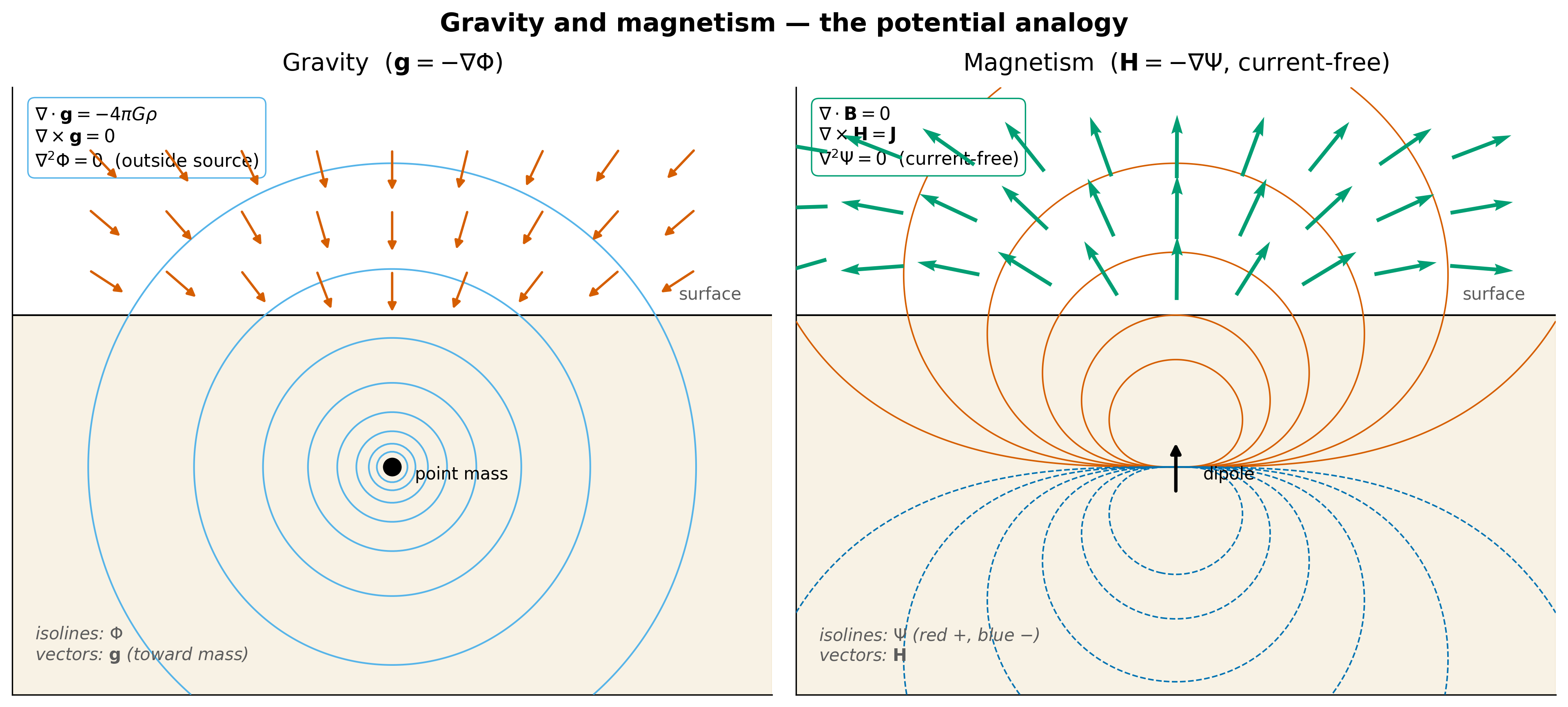— Fig. 118 Gravity and magnetism are both **potential fields** in source-free regions. The gravitational potential $\Phi$ obeys Laplace’s equation outside mass concentrations, and the magnetic scalar potential $\Psi$ (with $\mathbf{H} = -\nabla\Psi$) obeys Laplace’s equation outside free currents. The same upward- and downward-continuation operators apply to both — which is why the survey machinery of Lecture 21 transfers almost verbatim. The crucial *physical* difference is that mass is a positive scalar source, while magnetisation is a vector — a buried body produces a dipolar pattern that depends on both the body’s magnetisation direction and Earth’s ambient inducing field.#

Global lithospheric magnetic-anomaly poster from NOAA NCEI / CIRES, showing the EMAG2 v3 grid upward-continued to 4 km altitude on a Mercator projection. Anomaly intensity Delta F in nanoteslas is colour-coded with a diverging red-white-blue scale saturating at plus or minus 250 nT. Striped lineations parallel to mid-ocean ridges are visible across the Pacific, Atlantic, and Indian Oceans, recording 150 million years of seafloor spreading. The continents show long-wavelength patterns: a strong positive anomaly across the Canadian Shield and Greenland, a complex pattern over Africa and Antarctica, and the Mid-Continent Rift visible as a curving band through Minnesota and Iowa. A title strip and a colour-bar legend annotated in nT are integrated into the poster layout, together with a small inset of the polar caps. 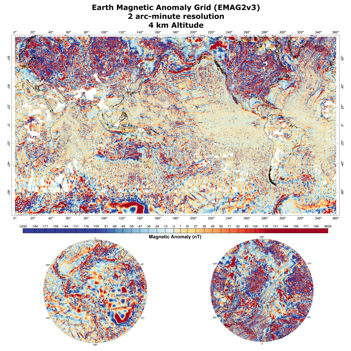— Fig. 119 The global lithospheric magnetic-anomaly grid, EMAG2 v3 [Meyer *et al.*, 2017], compiled from satellite, marine, and airborne measurements after removal of the core (IGRF) and external fields, and upward-continued to 4 km altitude. Anomaly magnitudes are reported in nT against a global ambient field of ~50 000 nT, so the colour scale represents perturbations of order $10^{-3}$ of the ambient. The map carries the fingerprint of 150 Myr of plate motion across the oceans and the full structural history of the continents. Source: NOAA NCEI / CIRES poster, US Government, public domain — original at https://www.ngdc.noaa.gov/geomag/data/EMAG2/EMAG2_V3_20170530/.#

The lecture works through this picture in three movements. Section 2 defines the magnetic anomaly $\Delta F$ and shows what physical signal it isolates. Sections 3–4 build the forward model for the simplest possible source — an induced dipole buried at depth — and explain why magnetic anomalies are asymmetric in a way that gravity anomalies are not. Sections 5–6 build the inverse problem (half-width depth, ensemble fit, the $m \propto z^3$ ridge, and the additional vector ambiguity from remanence). Section 7 reads three real anomaly maps at three scales — global EMAG2, continental USGS North America, and local Seattle Fault Zone — to illustrate what magnetic surveying is for.

2. What is a magnetic anomaly?#

A surface magnetometer measures the total intensity $F_\text{obs}(\mathbf{r}, t)$ of the magnetic field at position $\mathbf{r}$ and time $t$. From Lecture 23 §4, this measurement is the sum of three contributions from three depths:

(185)#\[F_\text{obs}(\mathbf{r}, t) = F_\text{core}(\mathbf{r}, t) + F_\text{lith}(\mathbf{r}) + F_\text{ext}(\mathbf{r}, t).\]

The core field $F_\text{core}$ is the dominant term (30 000–60 000 nT), generated by the geodynamo and modelled by the IGRF/WMM at any epoch. The lithospheric field $F_\text{lith}$ is static (~10 to ~1 000 nT) and is the signal of interest — the part of the measurement that carries information about subsurface structure. The external field $F_\text{ext}$ is time-varying (10–100+ nT on storm-quiet days, much larger during geomagnetic storms) and is a nuisance to be removed.

The total-field magnetic anomaly is what survives after the first and third contributions are subtracted:

(186)#\[\Delta F(\mathbf{r}) = F_\text{obs}(\mathbf{r}, t) - F_\text{IGRF}(\mathbf{r}, t) - F_\text{diurnal}(t).\]

Three operational corrections do the work of (186):

IGRF subtraction. The core-field value at the survey location and epoch is computed from the spherical-harmonic IGRF coefficients and subtracted point-by-point. This removes the long-wavelength core signal and the secular variation between survey years.
Base-station diurnal correction. A stationary magnetometer at the survey site records the time-varying external field continuously through the survey. Every roving measurement is corrected by subtracting the base-station value at the same time stamp. This removes the diurnal and storm variations.
Regional / IGRF-residual de-trending. Any low-order spatial trend remaining after IGRF removal (typically a linear or quadratic regional gradient) is fit and subtracted, leaving an anomaly map that integrates to zero over the survey area.

The signal that survives all three corrections is the lithospheric anomaly $\Delta F(\mathbf{r})$.

Schematic line plot showing the decomposition of a measured total-field signal into three components. The top trace, labelled F observed in nanoteslas, is a roughly constant baseline of about 52 000 nT with small bumps and a slow drift. Below it, three traces stack: the first labelled F IGRF (core field) is nearly constant at 52 800 nT with a slow downward trend; the second labelled F lithospheric is a static spatial perturbation of plus or minus 100 nT showing a localised positive peak above a buried body; the third labelled F external (diurnal) is a time-varying signal with diurnal swing of about 30 nT. A bottom panel labelled Delta F equals F obs minus F IGRF minus F diurnal shows the recovered lithospheric anomaly as a clean positive peak. 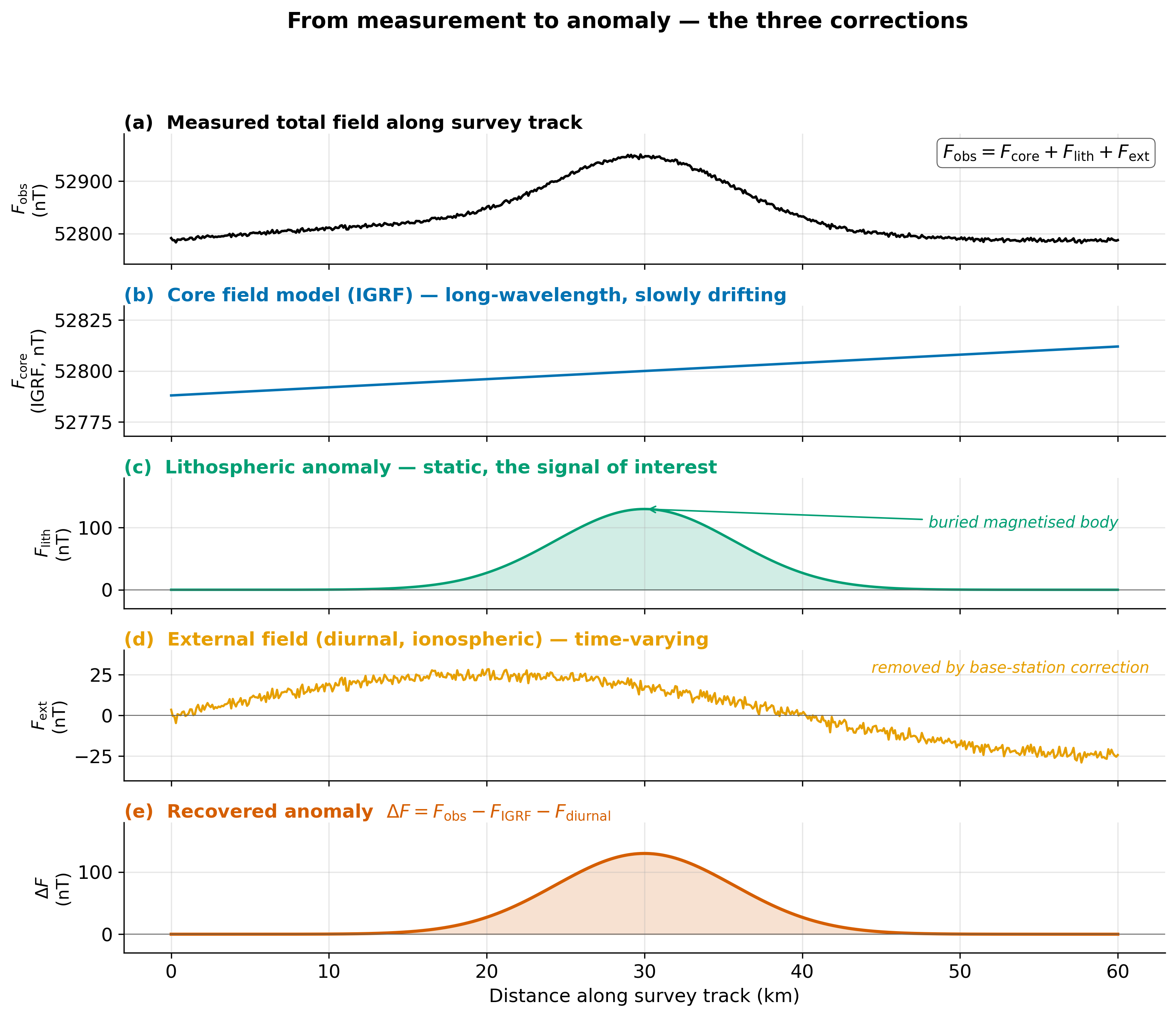— Fig. 120 The three-component decomposition of a surface magnetic measurement (185), and the operational extraction of the lithospheric anomaly $\Delta F$ via IGRF subtraction and diurnal correction. The measured signal $F_\text{obs}$ (top) is dominated by the core field $F_\text{core}$, with a small static perturbation from the lithospheric source and a time-varying perturbation from the ionosphere/magnetosphere. After removal of the IGRF model and the diurnal trace from a base station, the residual is the static lithospheric anomaly $\Delta F$ — the signal that carries information about buried magnetised bodies.#

The remainder of the lecture is about how the spatial pattern of $\Delta F(\mathbf{r})$ encodes the geometry, depth, and magnetisation of buried sources.

3. Forward problem — the buried induced dipole#

The simplest magnetic body that has a closed-form solution is a small sphere or compact volume of uniformly magnetised material — equivalent in its external field to a point magnetic dipole of moment $\mathbf{m}$. For a body in Earth’s ambient field, the dipole moment has two components:

(187)#\[\mathbf{m} = \mathbf{m}_\text{ind} + \mathbf{m}_\text{rem} = \chi V \mathbf{H}_\text{earth} + \mathbf{m}_\text{rem},\]

where $V$ is the body volume, $\chi$ is the volume magnetic susceptibility (Lecture 23 (175)), $\mathbf{H}_\text{earth}$ is the local ambient field (in A m$^{-1}$), and $\mathbf{m}_\text{rem}$ is the permanent (e.g. TRM) component — same subscript convention as L24 §3. For a freshly intruded volcanic body the two terms can be comparable; for an old plutonic body with low Königsberger ratio the induced term usually dominates. For the remainder of this section we restrict attention to the induced case, returning to the vector ambiguity in §6.

Place the dipole at $(0, z)$ with $z > 0$ measured downward, and the observation at $(x, 0)$ on the surface. The vector from source to observation is $\mathbf{r} = (x, -z)$ with $r = \sqrt{x^2 + z^2}$. The induced moment direction is $\hat{\mathbf{m}} = (\cos I, \sin I)$ — parallel to the inducing field with inclination $I$. The dipole field is

(188)#\[\mathbf{B}_\text{dipole} = \frac{\mu_0\, m}{4\pi}\,\frac{3(\hat{\mathbf{m}} \cdot \hat{\mathbf{r}})\hat{\mathbf{r}} - \hat{\mathbf{m}}}{r^3},\]

and the total-field anomaly is its projection onto $\hat{\mathbf{F}}_\text{earth} = \hat{\mathbf{m}}$:

(189)#\[\Delta F(x) = \mathbf{B}_\text{dipole}(x, 0) \cdot \hat{\mathbf{m}} = \frac{\mu_0\, m}{4\pi\, r^5}\,\bigl[3(\hat{\mathbf{m}}\cdot\hat{\mathbf{r}})^2 r^2 - r^2\bigr],\]

which can be expanded to give $\Delta F(x)$ explicitly in terms of $(x, z, I)$.

3.1 The shape of the anomaly depends on $I$#

The result of (189) is plotted in Fig. 121 for the same buried dipole evaluated at $I = 0$ (magnetic equator), $I = 45°$ (mid-latitude), and $I = 90°$ (magnetic pole).

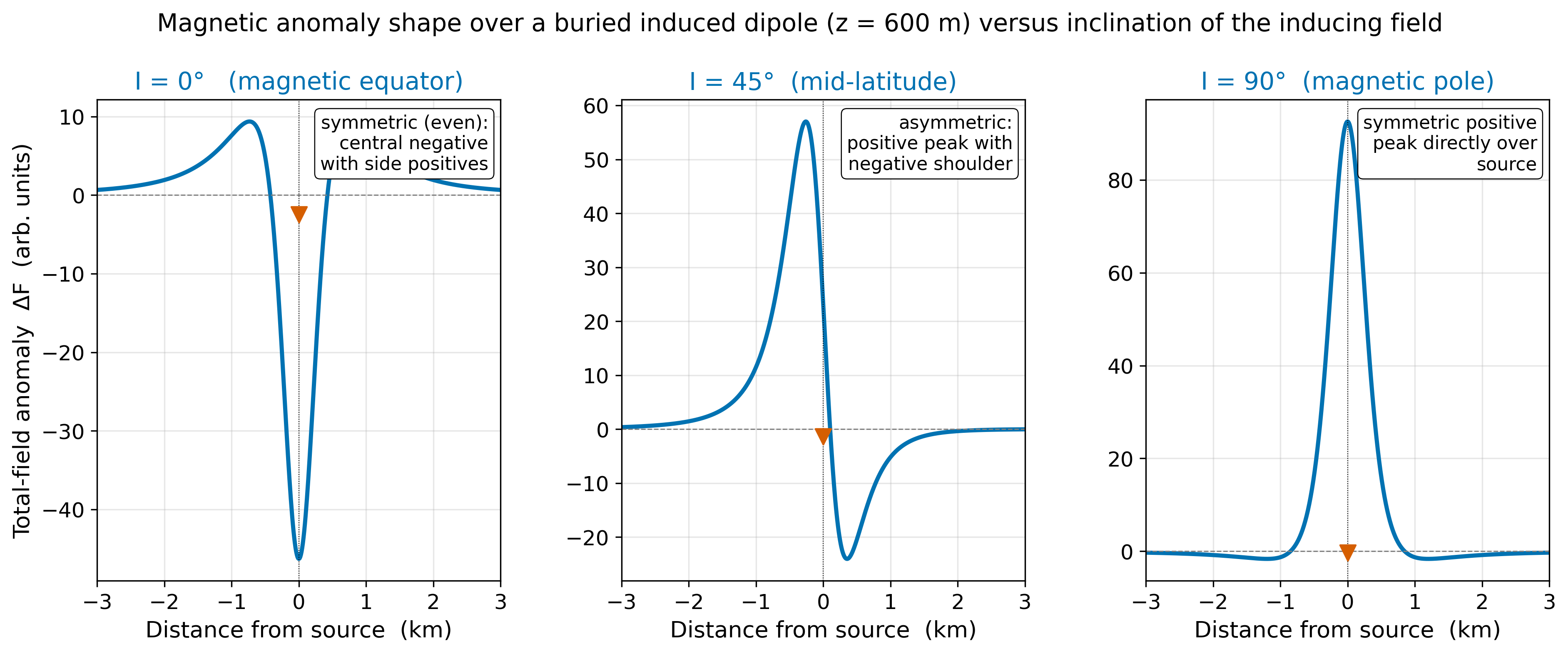
Fig. 121 Anomaly shape over a buried induced dipole at $z = 600$ m, as a function of the inclination of the inducing field. Magnetic equator ($I = 0$): symmetric “central negative + side positives” pattern. Mid-latitude ($I = 45°$): asymmetric profile, positive peak displaced toward the magnetic equator, with a small negative shoulder on the high-latitude side. Magnetic pole ($I = 90°$): symmetric positive peak directly over the source. Reproduces the qualitative content of Fig. 5.6 in [Blakely, 1995].#

The pole-symmetric case is the cleanest, and it is the geometry in which the half-width depth rule has its simplest form. At any other latitude, the asymmetric anomaly is harder to read — the apparent “centre” of the positive peak is not directly above the source. This is the central practical complication of magnetic versus gravity interpretation: gravity is always vertical, so a buried point mass always produces a symmetric peak centred above the source. The magnetic field at the source is not in general vertical, so the dipole orientation determines the anomaly shape. The standard processing step that fixes this is reduction to pole.

3.2 Reduction to pole#

Reduction-to-pole (RTP) is a frequency-domain filter that converts an anomaly measured at any $(I, D)$ into the anomaly that would have been measured at the magnetic pole. The filter is exact for an induced source whose direction of magnetisation equals the inducing-field direction, and approximate in general. Applied to a midlatitude anomaly, RTP centres the peak over the source and makes it symmetric (Fig. 122).

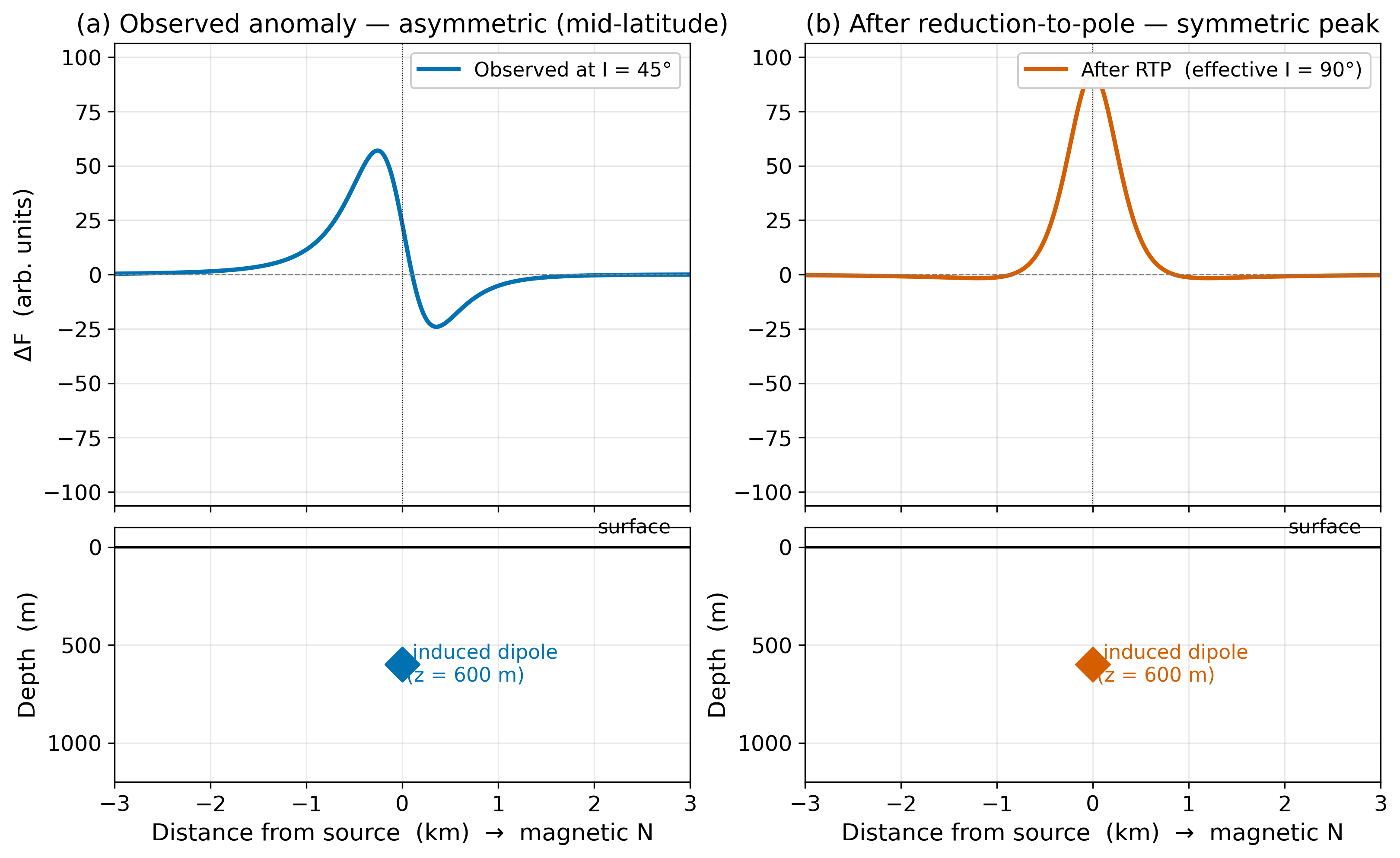
Fig. 122 Reduction-to-pole. (a) The asymmetric anomaly observed at mid-latitude ($I = 45°$) above the buried dipole is hard to centre by eye. (b) After RTP, the anomaly becomes a symmetric positive peak directly over the source — recovering the geometry that would have been measured at the magnetic pole. Both panels show the same subsurface body. Adapted from [Blakely, 1995], Section 12.3.#

For a Pacific-Northwest survey at $I \approx 69°$, the un-reduced anomaly is already mostly symmetric, and the practical benefit of RTP is modest. For a survey near the magnetic equator (Brazil, southeast Asia, equatorial Africa), the un-reduced anomaly is strongly asymmetric and RTP is essential.

4. The half-width depth rule#

At the pole (or after RTP), (189) reduces to

(190)#\[\Delta F(x) = \frac{\mu_0\, m}{4\pi}\, \frac{2 z^2 - x^2}{(x^2 + z^2)^{5/2}},\]

which has its maximum

(191)#\[\Delta F_\text{max} = \frac{\mu_0\, m}{4\pi}\, \frac{2}{z^3}\]

at $x = 0$ and falls to half its peak at

(192)#\[x_{1/2} \approx 0.5\, z, \qquad \text{equivalently} \qquad \boxed{\; z \;\approx\; 2\, x_{1/2}\;}\]

(Fig. 123b). The factor 0.5 is exact for an induced point dipole at the pole and approximate for any other geometry; it follows from solving $\Delta F(x_{1/2}) = \Delta F_\text{max} / 2$ in (190). Compared with the corresponding rule for the gravity sphere, $x_{1/2}^\text{grav} \approx 0.766\, z$ (Lecture 20, §3.4), the magnetic rule has a smaller prefactor — the magnetic anomaly falls off faster than the gravity anomaly because the dipole field decays as $r^{-3}$ rather than $r^{-2}$.

Three stacked panels. Panel a is a cross-section showing three diamond markers at the same horizontal position x equals 0 but at depths of 300 m blue, 600 m orange, and 1200 m green, with an orange vertical down-arrow labelled F earth vertical at pole on the left side. Receiver triangles are spaced along the surface line. Panel b is a plot of normalised delta F over delta F max versus horizontal distance from minus 3 to plus 3 km, showing three peaked curves; the z equals 300 m curve is narrow, the z equals 600 m intermediate, and the z equals 1200 m wide. A dotted horizontal line at 0.5 is labelled half peak; markers and annotations indicate half-widths of x half equals plus or minus 150 m for z equals 300 m, plus or minus 300 m for z equals 600 m, and plus or minus 600 m for z equals 1200 m. Panel c is a plot of total-field anomaly in nT versus horizontal distance for the deepest case z equals 1200 m only, showing a green Gaussian-like peak of 50 nT, a grey shaded horizontal band between minus 4 and plus 4 nT labelled plus or minus 2 sigma noise band sigma equals 2 nT, a dotted horizontal line at 25 nT labelled half peak equals 25 nT, and two vertical dashed lines at plus or minus 600 m connected by a double-headed arrow labelled 2 x half approximately 1200 m. An inset box reports inferred z equals 1200 m, S over N at peak equals 25, sigma z over z approximately 1.3 percent, sigma z approximately 16 m. 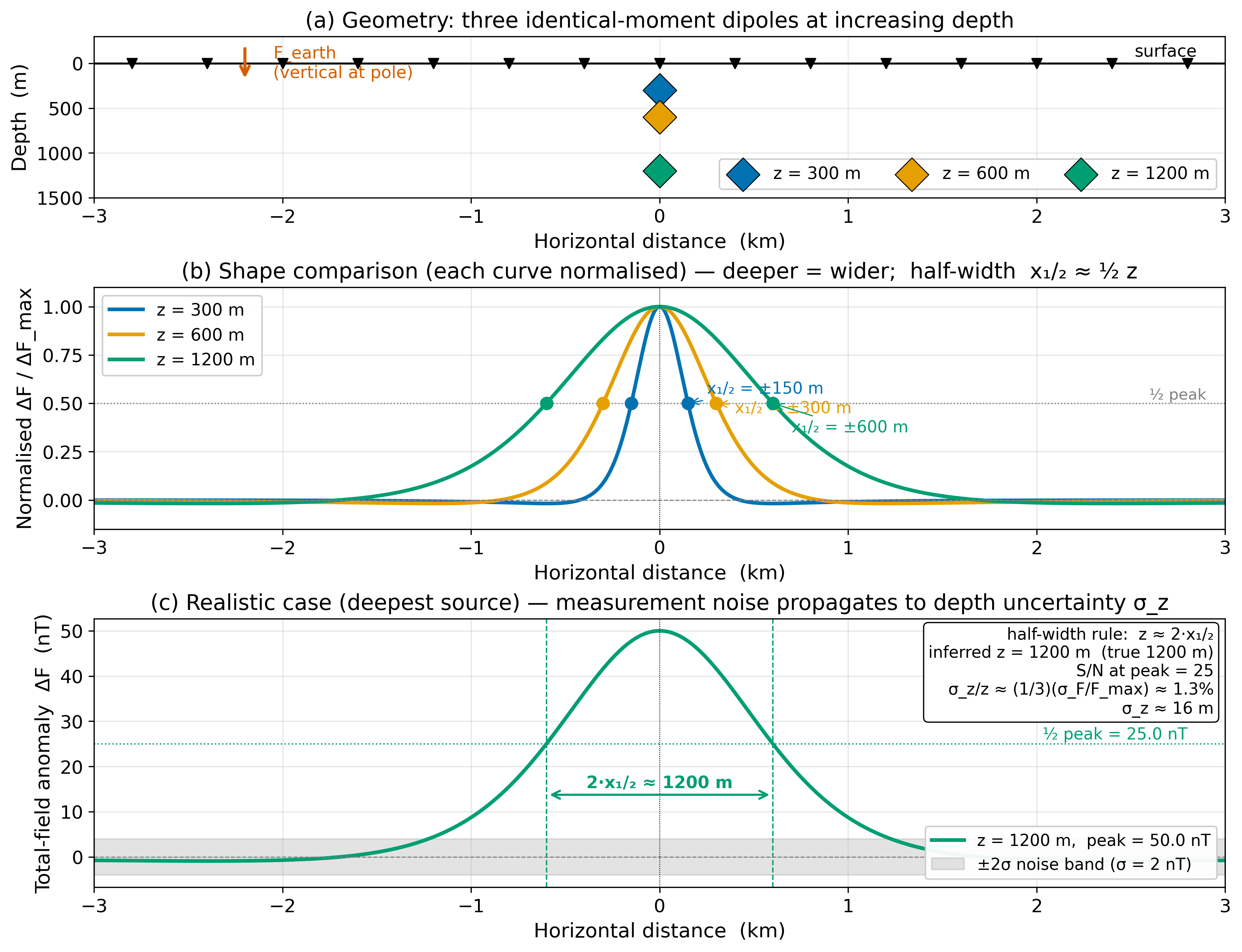— Fig. 123 The half-width depth rule, with measurement-noise propagation. **(a)** Three identical-moment dipoles at $z = 300, 600, 1200$ m. **(b)** The same anomalies normalised by their peaks — deeper sources produce wider profiles. The half-width $x_{1/2}$ scales linearly with $z$. **(c)** For the deepest source, the realistic peak amplitude is 50 nT; a $\pm 2\sigma$ noise band of $\sigma = 2$ nT (typical of a regional aeromagnetic survey) gives a signal-to-noise ratio of 25 at the peak. The inferred depth $z = 2\,x_{1/2} = 1200$ m matches truth. Propagating $\sigma_F = 2$ nT through the half-width formula gives $\sigma_z \approx 16$ m, or roughly 1% of the depth — see §4.1.#

4.1 Measurement errors and the noise → depth chain#

The half-width rule (192) is exact for clean data, but real magnetic surveys are noisy at several stages:

Sensor noise. A proton-precession magnetometer measures total field by precession of proton magnetic moments; sensor noise is roughly 0.1 nT in a single one-second reading. Cesium-vapour magnetometers (the standard for high-resolution aeromagnetics) achieve 0.01 nT. Both are far below the typical anomaly amplitudes of interest.
Positioning error. Modern GPS gives a station location to ~1 m horizontally — small compared with the survey-line spacing of 100 m–1 km that ordinarily controls the spatial resolution of an anomaly map.
External (diurnal) variation. Earth’s external field changes by 10–50 nT during a typical day, with much larger swings during magnetic storms. This is the dominant source of error in a magnetic survey and is removed by a base-station correction (§2). Surveys are also designed to cross over themselves (looped traverses) so that any residual drift can be estimated from the closure error.
Regional gradients and the IGRF. The main field varies on the scale of hundreds of kilometres. For a survey of a few-km extent, an affine regional trend is subtracted; for a continental-scale survey, the IGRF model is removed point by point.

After all corrections, a typical regional aeromagnetic survey delivers total-field anomalies with $\sigma_F \approx$ 1–5 nT. To translate this into a depth uncertainty, note that the peak amplitude in (191) depends on $z$ as $\Delta F_\text{max} \propto z^{-3}$. Differentiating the half-width rule (192) with respect to the measured peak gives, at fixed $m$:

(193)#\[\frac{\sigma_z}{z} \;\approx\; \frac{1}{3}\,\frac{\sigma_F}{\Delta F_\text{max}}.\]

The factor 1/3 in (193) is the analog of the 1/2 factor in the gravity formula (Lecture 20, eq. 3.6.4), and it is smaller because the magnetic field falls off more steeply with distance. For a fixed signal-to-noise ratio, magnetic depths are inferred more precisely than gravity depths — provided one stays in the regime of induced-only magnetisation.

SNR rule of thumb

$\Delta F_\text{max} / \sigma_F$	Depth uncertainty $\sigma_z / z$	Verdict
> 50	< 0.7%	Excellent — depth pinned.
10 – 50	0.7% – 3%	Good — depth well-constrained.
< 10	> 3%	Poor — quote bounds, not a number.

For the example in Fig. 123c, SNR = 25 gives $\sigma_z / z = 1.3\%$, or $\sigma_z = 16$ m on a 1 200 m source — better than the depth resolution of most seismic-reflection surveys at that depth.

5. Inverse problem — the ensemble fit and the $m \propto z^3$ ridge#

The half-width rule gives a single best-fit depth and a single propagated uncertainty, but it commits to the form of the source (a point induced dipole at the pole) before reading the data. A more honest treatment is to scan over the full $(z, m)$ parameter space, compute the $\chi^2$-misfit of the predicted profile against the observations, and accept every model whose reduced $\chi^2$ falls below a threshold — the same protocol used in Lecture 20 §3.7 for the gravity sphere.

The result is the ensemble cloud in Fig. 124. The accepted models — those with $\chi^2/N \leq 1.5$, given $\sigma_F = 2$ nT and 31 stations — line up along a curved valley in $(z, m)$ space:

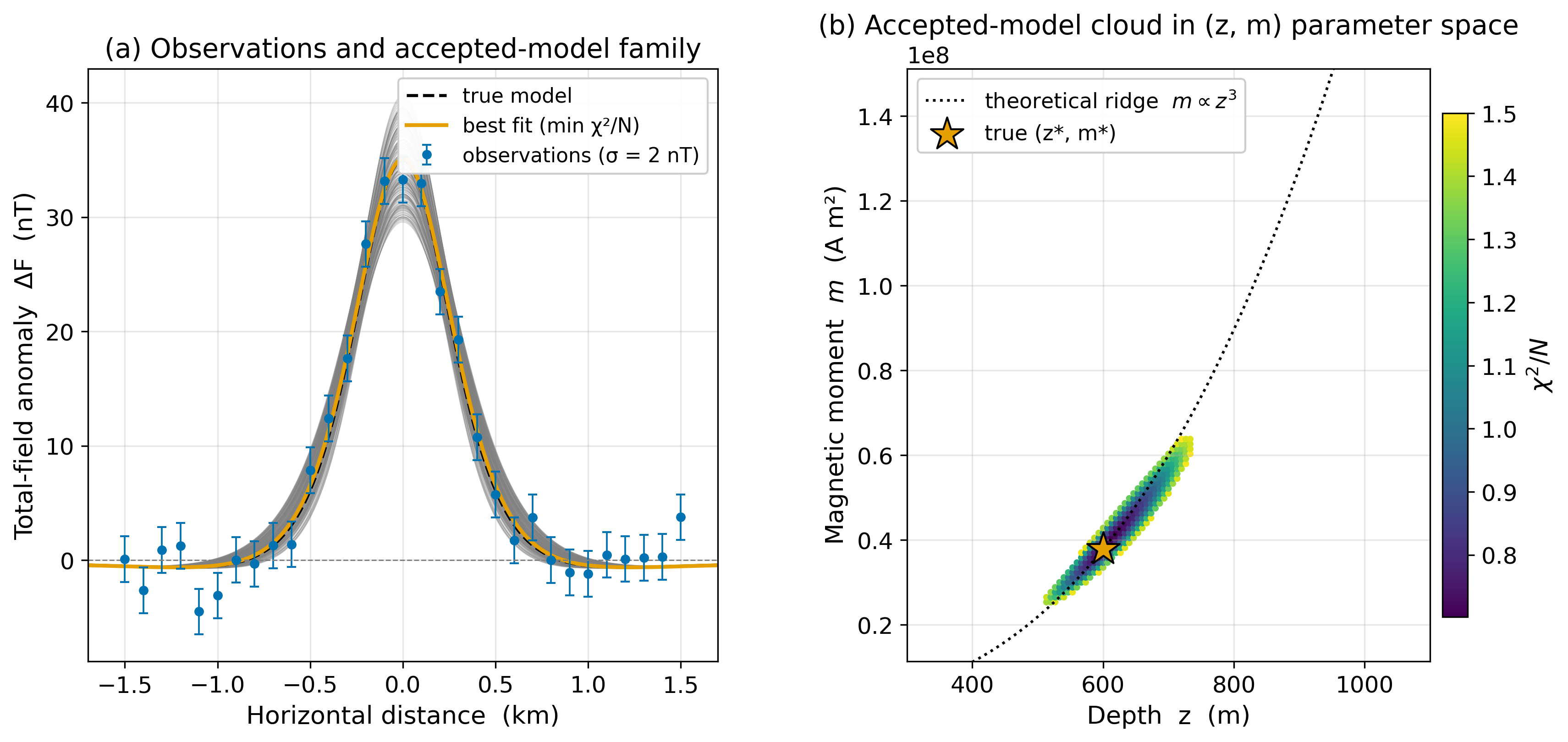
(194)#\[m \;\propto\; z^3 \qquad \text{(magnetic ridge, induced point dipole, at the pole)}.\]

Fig. 124 From data error to model uncertainty for the induced point dipole at the pole. (a) 31 synthetic stations with $\sigma_F = 2$ nT, the true model (dashed), the best-fit minimum-$\chi^2$ model (orange), and 200 randomly selected accepted models (grey). (b) The accepted models in $(z, m)$ space, coloured by reduced chi-squared. The cloud lies along the theoretical $m \propto z^3$ ridge, which is the magnetic analog of the $M \propto z^2$ ridge for a gravity sphere. The depth and the moment are strongly correlated; neither can be pinned down independently from peak amplitude alone — only the combination $m/z^3$ is.#

The ridge (194) has a steeper exponent than the gravity case ($M \propto z^2$) because the magnetic field decays as $r^{-3}$. The depth-moment correlation is therefore stronger in the magnetic case: a 10% error in inferred depth translates into a 30% error in inferred moment. The half-width measurement breaks this degeneracy by constraining the width of the profile in addition to its amplitude — hence the importance of having stations spaced finely enough to resolve $x_{1/2}$, not merely the peak.

6. A complication unique to magnetics — the induced/remanent ambiguity#

For a gravity survey, the only physical ambiguity in inversion is the trade-off between source mass and depth: a deep heavy source produces the same anomaly as a shallow light one. For a magnetic survey, two ambiguities operate together:

The same $(z, m)$ trade-off, intensified to $m \propto z^3$ (§5).
An additional vector ambiguity in the magnetisation direction: $\mathbf{m} = \mathbf{m}_\text{ind} + \mathbf{m}_\text{rem}$ (187). The induced component is parallel to $\mathbf{H}_\text{earth}$, but the remanent component can point in any direction — its orientation was set when the body last cooled through the Curie temperature, possibly at a different geographic latitude (paleo-latitude, Lecture 23 §7), possibly during a different polarity epoch (the GPTS, Lecture 24 §6).

The consequence is that a single magnetic-anomaly profile cannot, in general, separate induced from remanent magnetisation. If a body is known to be young and felsic ($Q \ll 1$, Lecture 24 §3), the induced-only assumption is safe. If the body is volcanic and recent ($Q \gg 1$, e.g. fresh basalt), the induced-only assumption fails spectacularly.

Resolution requires more data: gradiometry to constrain the direction of $\mathbf{B}_\text{source}$ at multiple stations, laboratory measurements of representative samples for the bulk $\mathbf{M}_\text{rem}$ and $Q$, or joint inversion with gravity (which sees only mass and is blind to remanence). All three approaches are in standard use today, and the third is the cleanest example of multi-physics integration in shallow-Earth geophysics: combining two observables that share the depth-extent of the source but differ in their sensitivity to the source’s physical properties.

7. Reading real anomaly maps at three scales#

The same governing physics — a magnetised body $\mathbf{m}$ at depth $z$ producing a surface perturbation $\Delta F$ via (189) — operates from a 30-m drone survey of a fault scarp up to a 460-km-altitude satellite mapping the lithospheric field globally. The three scales of magnetic anomaly maps resolve three different geological scales of structure.

7.1 Continental scale — USGS North America#

The USGS Magnetic Anomaly Map of North America [Bankey et al., 2002] is a continental-scale compilation of aeromagnetic surveys, gridded at ~1 km resolution and corrected to a common datum. The map resolves the structural fabric of every major Precambrian shield, every Phanerozoic orogen, and every continental-margin basin in North America — the geological architecture of an entire continent in a single image (Fig. 125).

Continental magnetic anomaly map of North America in colour, showing diverging blue and red anomalies on a base map of state and provincial boundaries. The map shows a strong positive anomaly pattern across the Canadian Shield in central and eastern Canada, complex linear trends across the Appalachians, the Mid-Continent Rift visible as a curving north-south band of strong positive anomaly through Minnesota and Iowa, and varied anomaly patterns across the western Cordillera. The Pacific Northwest region is annotated with a small inset highlighting the Cascadia subduction zone and Olympic Peninsula. 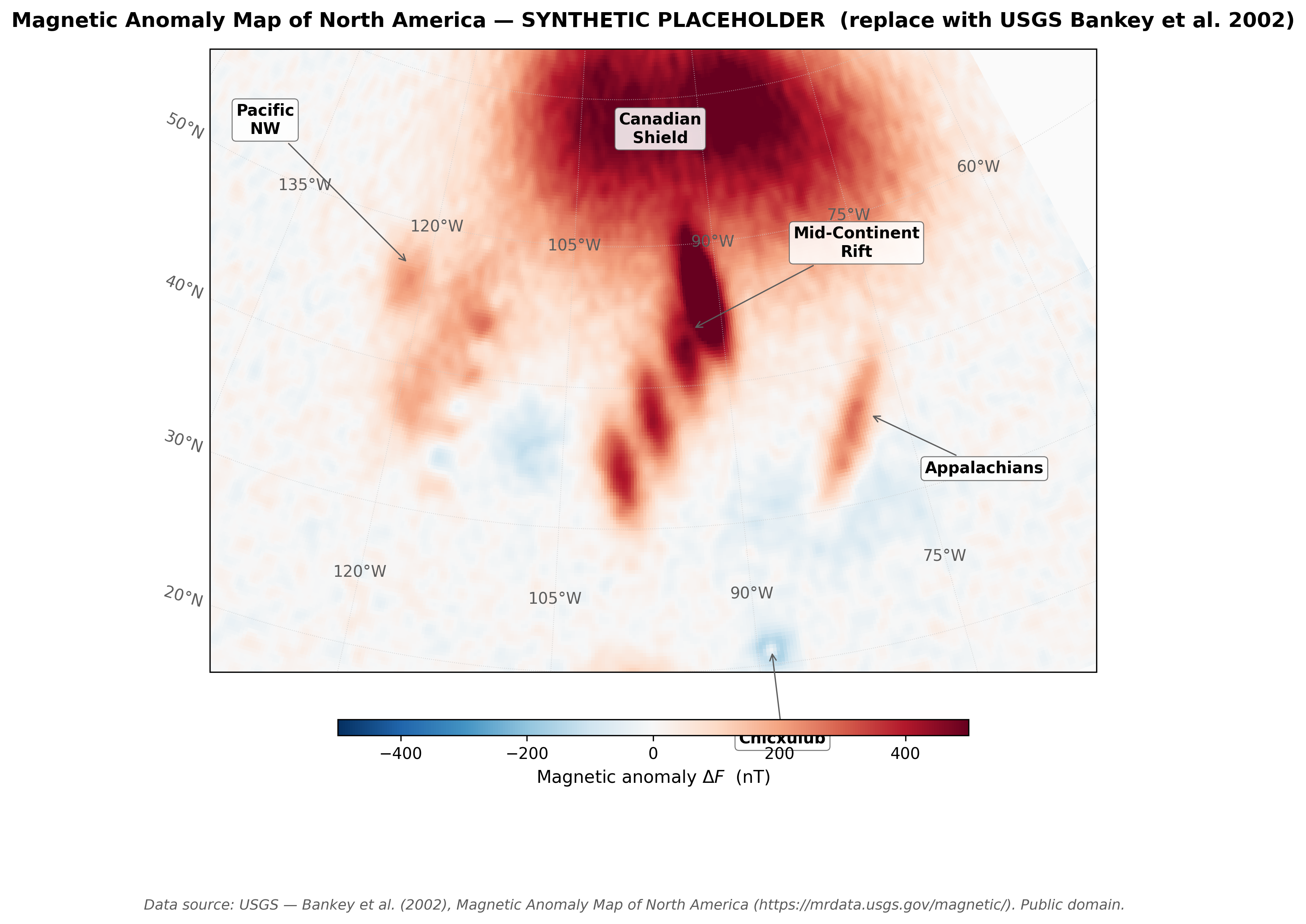— Fig. 125 The Magnetic Anomaly Map of North America [Bankey *et al.*, 2002], gridded at 1 km resolution from compiled aeromagnetic surveys. The image is the surface signature of the upper ~30 km of the lithosphere: the long-wavelength positive anomaly through the Canadian Shield outlines Archean and Paleoproterozoic crust; the Mid-Continent Rift (a 1.1-Ga failed rift through Minnesota and Iowa) is one of the strongest signatures on the map; the Pacific Northwest carries a complex pattern dominated by the accreted Siletzia terrane (Lecture 24 §8) and the Cascade arc volcanics. Source: USGS, US Government, public domain.#

7.2 Local scale — the Seattle Fault Zone from the air#

In the Pacific Northwest, magnetic methods are central to one of the most consequential applied-geophysics projects of the past quarter century: high-resolution aeromagnetic mapping of the Seattle Fault Zone (SFZ), an east-west zone of active blind reverse faults that crosses Puget Sound directly beneath downtown Seattle and Bainbridge Island.

The SFZ was first recognised from paleoseismic trenching and LIDAR-imaged fault scarps; it was placed on the regional geophysical map by a 1997 USGS aeromagnetic survey at 300-m line spacing [Blakely et al., 2002]. Tertiary volcanic units of the Crescent Formation — part of the Siletzia terrane (Lecture 24 §8) — are uplifted on the hanging wall and produce strong positive magnetic anomalies (peaks of several hundred nT). The magnetic contrast against the sedimentary footwall of the Seattle basin defines a sharp linear edge that traces the fault for tens of kilometres beneath the urban surface (Fig. 126).

Map of the Seattle metropolitan area showing a magnetic anomaly map overlaid on streets and shorelines. The map covers approximately 47.4 to 47.7 degrees north latitude and 122.6 to 122.2 degrees west longitude, including Bainbridge Island on the west, downtown Seattle in the centre, and Lake Washington on the east. A linear east-west zone of strong positive anomaly (peak amplitudes plus 200 to plus 500 nT) runs across the centre of the map at approximately 47.6 degrees north, with a sharp gradient on its north side. The positive anomaly is interpreted as the uplifted Crescent Formation volcanic units in the hanging wall of the Seattle Fault Zone. Streets and shorelines are overlaid for geographic reference. 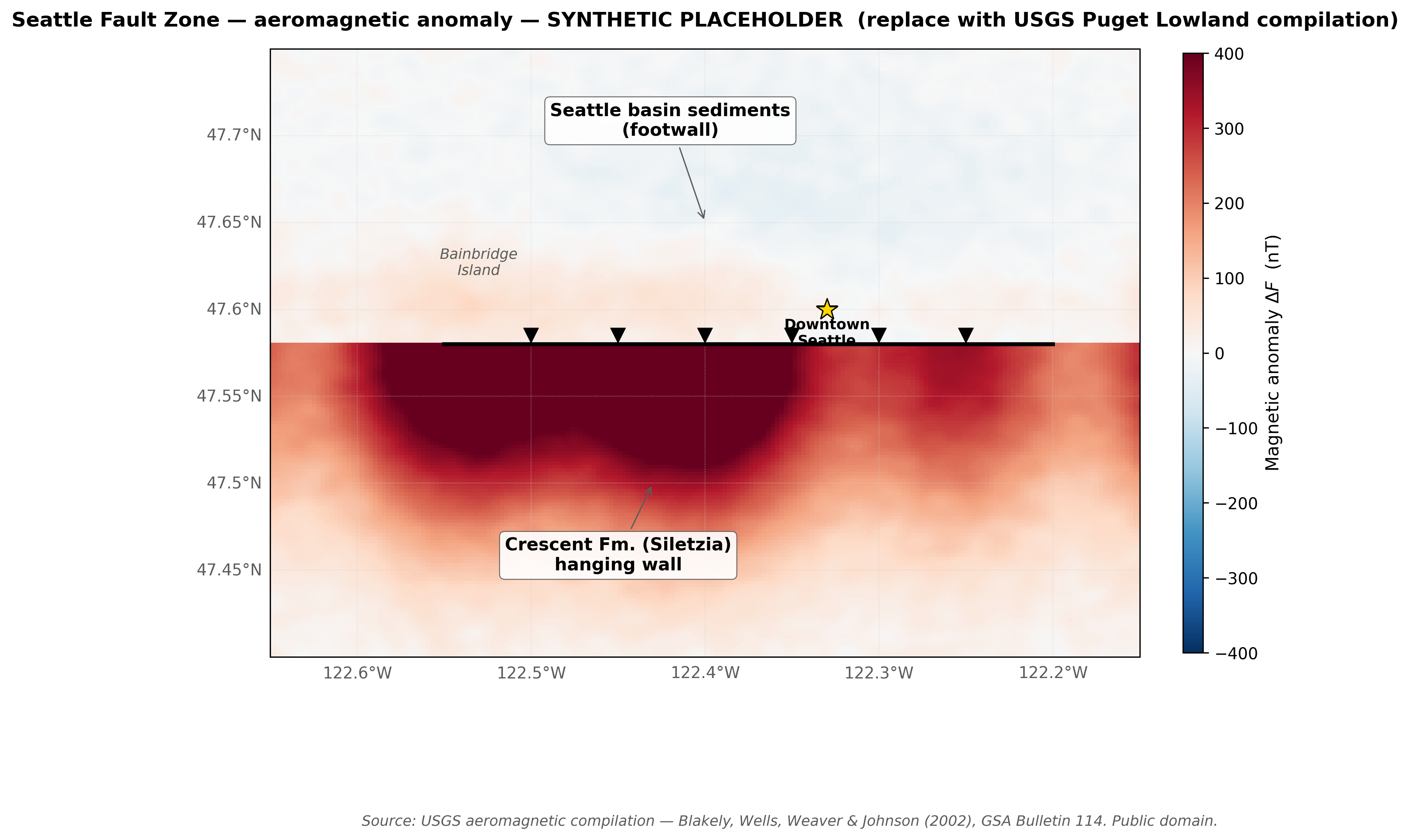— Fig. 126 The Seattle Fault Zone in magnetic-anomaly map view, after [Blakely *et al.*, 2002]. The east-west zone of strong positive anomaly across central Puget Sound and downtown Seattle marks the uplifted Crescent Formation basalts (Eocene Siletzia volcanic units) on the hanging wall of the blind reverse fault. The sharp gradient on the north side of the anomaly is the surface expression of the fault plane — a 30-km-long structure dipping south under Bainbridge Island, downtown Seattle, and Mercer Island. The maximum credible earthquake on this structure is approximately $M_w$ 7. Source: USGS aeromagnetic compilation, US Government, public domain.#

The maximum earthquake credible on the SFZ is approximately $M_w$ 7 — large enough to cause heavy damage in downtown Seattle, with shaking amplified by the soft sediments of the Seattle basin. The Washington State seismic hazard maps used by code authorities for building design lean directly on the fault geometry recovered from the aeromagnetic survey. Magnetic methods cannot identify when the next earthquake will occur, but they can — and do — establish where it is most likely to nucleate, which is the prior input to every probabilistic hazard calculation.

7.3 Why three scales matter#

The anomaly $\Delta F$ at any point is the integrated contribution of all magnetised bodies in the lithosphere beneath the survey location. The scale of the survey selects which sources dominate the recovered signal — through the spatial-wavelength filtering already discussed in Lecture 23 §4.4:

Survey scale	Spatial wavelength resolved	Geological feature scale	Typical use
Satellite (Swarm)	≥ 300 km	Continental shields, large impacts	Global lithospheric mapping
Aeromagnetic (regional)	1–30 km	Plutons, ridges, large faults	Tectonic mapping, mineral exploration
Aeromagnetic (high-res, drone)	10 m – 1 km	Dykes, faults, archaeological features	Detailed hazard mapping, UXO clearance
Ground (magnetometer + GPS)	< 10 m	Individual ore bodies, buried metal	Mineral grade control, environmental forensics

In practice a study at one scale is often only a step in a hierarchy: an aeromagnetic compilation flags a regional feature, a high-resolution drone survey resolves its near-surface geometry, and ground-truth samples discriminate the induced from the remanent contribution. The Seattle Fault story is exactly this — a regional aeromagnetic survey placed the fault on the map; follow-on high-resolution work resolved individual fault strands; rock-magnetic samples of the Crescent Formation constrained the source magnetisation; joint inversion with gravity bounded the depth of the buried hanging-wall structure.

8. Research horizon — magnetic methods today#

The 60-year-old Vine–Matthews–Morley framework (Lecture 24) still grounds magnetic interpretation, but the modern frontier sits in four places:

Joint magnetic–gravity inversion for ore-deposit exploration (gold, nickel sulfide, lithium pegmatites, rare-earth elements): combined sensitivity to density and magnetisation breaks ambiguities that neither dataset resolves on its own.
UAV-borne magnetics: drone-mounted total-field and gradient magnetometers now achieve 0.05 nT precision at 30 m line spacing, delivering near-surface anomaly maps once limited to ground surveys. UAV traverses over hidden faults on Bainbridge Island have piloted a hazard-mapping application directly relevant to Puget Sound urban resilience.
Machine-learning inversion. Deep-learning surrogate models have begun to replace the bulk of the forward simulations in iterative inversion, but every surrogate so far in production use is trained on physics-based simulations of the dipole-Maxwell equations of §3. The neural network is a substitute for the matrix-vector multiplication, not for the physics.
Planetary magnetism. Crustal remanence mapped by Mars Global Surveyor, MAVEN, and Mercury’s MESSENGER has revealed that Mars carried a strong dynamo until ~3.7 Ga and that Mercury’s small dipole is still active. The same inversion tools — Lecture 25’s induced-dipole forward operator, the half-width depth rule, ensemble fitting — applied to satellite data over silent dynamos.

9. AI literacy — the latitude trap#

A common failure mode of large language models on magnetic-anomaly problems is to treat the anomaly shape as if the survey were always at the pole — that is, to ignore the latitude dependence of the forward problem.

AI Epistemics activity

Step 1. Sketch (by hand, on graph paper) a magnetic anomaly profile over a small buried induced dipole at three different latitudes: the magnetic pole, a mid-latitude site at $I = 45°$, and the magnetic equator. Use Fig. 121 as a guide if needed.

Step 2. Hand the equator profile (only — without telling the LLM where it was measured) to a chat model and ask it to infer the depth of the source using the half-width rule.

Step 3. Check whether the LLM:

Asks for the latitude before applying the half-width rule. (Good.)
Applies the half-width rule directly. (Bad — the rule does not work without RTP.)
Generates a confidently wrong number. (Worst.)

Step 4. Whichever the case, write a single-paragraph rebuttal that either (i) explains why your LLM’s question for the latitude was appropriate, or (ii) demonstrates that the LLM’s answer is wrong by deriving the correct procedure (RTP first, then half-width).

The deliverable is the LLM transcript + your rebuttal. The grading criterion is not whether the LLM was right, but whether you caught the error and could defend the correct procedure.

10. Concept check#

Concept-check questions

Half-width and SNR. A regional aeromagnetic survey over a basalt plug at the magnetic pole gives a peak anomaly of $\Delta F_\text{max} = 80$ nT with surveyed half-width $x_{1/2} = 240$ m and a measurement noise of $\sigma_F = 4$ nT. Compute the depth using the half-width rule, the SNR, and the propagated depth uncertainty from (193). Is this an “excellent / good / poor” determination by the rule of thumb in §4.1?
Reading the asymmetry. A magnetic anomaly profile in eastern Oregon (geomagnetic inclination $I \approx +66°$) shows a positive peak that is offset $\sim 150$ m to the south of the apparent surface trace of a known buried body. Is this offset consistent with an induced-only source? In which direction (north or south) does the asymmetry of the un-reduced anomaly displace the peak relative to the source, at northern-hemisphere latitudes?
Induced or remanent? A small buried body in eastern Oregon produces a strongly negative magnetic anomaly at a station above it (peak $\Delta F = -200$ nT) — the opposite sign from what would be expected for an induced dipole at $I = +69°$. Sketch two physical scenarios that could produce this signature. Which additional measurement would you make to discriminate between them?
Joint inversion intuition. A buried body produces a $+150$ nT magnetic anomaly and a $+0.5$ mGal gravity anomaly at the surface. (a) Use the magnetic half-width rule (assuming pole geometry) and the gravity half-width rule from Lecture 20 to obtain two independent depth estimates. (b) Suppose they disagree by 30%. Name three physical factors that could cause this disagreement, and explain which would shift the magnetic estimate, which would shift the gravity estimate, and which would shift both.

Concept-check answers

Answers and worked solutions are provided in the instructor materials (see concept_check_lecture25.md in the ess314-instructor repository).

11. Looking ahead#

Lecture 25 closes the magnetism module of ESS 314. Module 7 — Geodynamics and Tectonics — opens at Lecture 26 with Heat and Geodynamics: the planetary heat budget, the thermal structure of the lithosphere, the rheology of the asthenosphere, and the driving forces of plate motion. The bridge from this lecture to the next is the Curie isotherm itself: rocks below the Curie temperature carry remanence and contribute to the lithospheric anomaly; rocks above lose their order and are magnetically silent. The depth at which Earth’s geotherm crosses the Curie isotherm — typically 20–40 km in continental crust, much shallower under mid-ocean ridges and arcs — is therefore the physical lower bound of the lithospheric magnetic source layer. The same geotherm controls strength, rheology, partial melting, and the dynamics of plate boundaries, and that’s where the synthesis module begins.

12. Further reading#

Open-access references are preferred; paywalled works are cited for completeness but are not required for the lecture.

[1] (1,2)

V. Bankey, A. Cuevas, D. Daniels, C. A. Finn, I. Hernandez, P. Hill, R. Kucks, W. Miles, M. Pilkington, C. Roberts, W. Roest, V. Rystrom, S. Shearer, S. Snyder, R. Sweeney, J. Velez, J. D. Phillips, and D. Ravat. Digital data grids for the magnetic anomaly map of North America. 2002. URL: https://mrdata.usgs.gov/magnetic/, doi:10.3133/ofr02414.

[2] (1,2)

Richard J. Blakely. Potential Theory in Gravity and Magnetic Applications. Cambridge University Press, Cambridge, UK, 1995. ISBN 978-0521415088. doi:10.1017/CBO9780511549816.

[3] (1,2)

Richard J. Blakely, Ray E. Wells, Craig S. Weaver, and Samuel Y. Johnson. Location, structure, and seismicity of the Seattle fault zone, Washington: evidence from aeromagnetic anomalies, geologic mapping, and seismic-reflection data. Geological Society of America Bulletin, 114(2):169–177, 2002. doi:10.1130/0016-7606(2002)114<0169:LSASOT>2.0.CO;2.

[4]

S. Maus. The geomagnetic power spectrum. Geophysical Journal International, 174(1):135–142, 2008. doi:10.1111/j.1365-246X.2008.03820.x.

[5]

B. Meyer, R. Saltus, and A. Chulliat. EMAG2: Earth Magnetic Anomaly Grid (2-arc-minute resolution), version 3. 2017. Public domain dataset. URL: https://www.ncei.noaa.gov/products/earth-magnetic-anomaly-grid-2-arc-minute-resolution, doi:10.7289/V5H70CVX.

Companion notebook (next step)

The accompanying Jupyter notebook magnetics_ensemble.ipynb (in the course notebooks/ directory) implements the forward operator of §3 and the ensemble grid-search of §5, and asks students to invert a synthetic anomaly profile for source depth and moment. Lab 8 extends this to a real Pacific Northwest aeromagnetic profile and includes a reduction-to-pole step. A companion notebook magnetics_forward.ipynb (introduced with Lecture 23) supplies the IGRF/WMM field-calculator that students use as a baseline for the IGRF-subtraction step of §2.

Open data and tools

USGS Aeromagnetic Compilations: https://mrdata.usgs.gov/magnetic/ — open access to all US Government aeromagnetic surveys at the continental, state, and 7.5’-quadrangle scales.
NOAA NCEI EMAG2 v3: https://www.ncei.noaa.gov/products/earth-magnetic-anomaly-grid-2-arc-minute — the global lithospheric anomaly grid used in §1, public domain, gridded at 2 arc-minutes.
NOAA NCEI Marine Trackline Geophysics: https://www.ncei.noaa.gov/maps/trackline/ — ship-towed marine magnetic profiles, public domain.
PyGMI (Python Geophysical Modelling Interface): Patrick-Cole/pygmi — open-source 2D/3D potential-field forward modelling and inversion.
SimPEG: https://www.simpeg.xyz/ — open-source simulation and parameter-estimation framework for geophysics, including magnetics.


Course LOs addressed	LO-1 (observables ↔ Earth properties), LO-2 (forward model), LO-3 (inverse problem with \(d = G(m)\)), LO-4 (uncertainty and non-uniqueness), LO-5 (multi-physics integration with gravity and seismic reflection)
Learning outcomes practiced	LO-OUT-A (forward problem from governing equation), LO-OUT-B (inverse problem with model uncertainty), LO-OUT-D (multi-physics interpretation), LO-OUT-E (societal-relevance reasoning, via the Seattle Fault aeromagnetic survey)
Prior lecture	L24 — Rock Magnetism: How Rocks Remember the Field
Next lecture	L26 — Heat and Geodynamics
Lab connection	Lab 8 — Magnetic Anomaly Inversion (ensemble fit of an induced dipole; reduction to pole; interpretation of a real Pacific Northwest profile)
Textbook	Lowrie & Fichtner (2020), Ch. 5.4–5.7

Symbol	Name	Units / notes
\(F_\text{obs}\)	Total intensity measured at a survey station, $F_\text{obs}=	\mathbf{B}
\(F_\text{core}\)	Core-field contribution to \(F_\text{obs}\) (the geodynamo signal, L23 §4).	nT
\(F_\text{lith}\)	Lithospheric contribution (the signal of interest for surveying).	nT
\(F_\text{ext}\)	External (ionospheric / magnetospheric) contribution.	nT
\(F_\text{IGRF}\)	Modelled core field from the IGRF at the survey epoch (subtracted from \(F_\text{obs}\)).	nT
\(F_\text{diurnal}\)	Base-station time-varying trace used to remove the external field.	nT
\(\Delta F\)	Total-field magnetic anomaly: \(\Delta F = F_\text{obs} - F_\text{IGRF} - F_\text{diurnal}\).	nT
\(\Delta F_\text{max}\)	Peak amplitude of \(\Delta F\) at the surface above the source.	nT
\(\sigma_F\)	RMS measurement noise on \(\Delta F\) after all corrections.	nT
\(\mathbf{m}\)	Dipole moment of a buried body (local to L25; distinct from Earth’s \(\mathbf{m}\) in L23).	A m\(^2\)
\(\mathbf{m}_\text{ind},\,\mathbf{m}_\text{rem}\)	Induced and remanent components of the body moment: \(\mathbf{m} = \chi V \mathbf{H}_\text{earth} + \mathbf{m}_\text{rem}\).	A m\(^2\)
\(V\)	Volume of the buried body.	m\(^3\)
\(\mathbf{F}_\text{earth},\,\hat{\mathbf{F}}_\text{earth}\)	Local ambient total-field vector and its unit direction at the survey point.	nT, —
\(\mathbf{B}_\text{source}\)	Surface field perturbation produced by a buried magnetised body.	nT
\(\mathbf{B}_\text{dipole}\)	Closed-form dipole field of the body — eq. (188).	nT
\(\mathbf{r},\,r\)	Vector from source to observation, and its magnitude.	m
\(\hat{\mathbf{m}},\,\hat{\mathbf{r}}\)	Unit vectors of \(\mathbf{m}\) and \(\mathbf{r}\).	—
\(x,\,z\)	Horizontal surface coordinate and depth-below-surface (positive downward).	m
\(x_{1/2}\)	Half-width of the anomaly: \(\Delta F(x_{1/2}) = \tfrac12\Delta F_\text{max}\).	m
\(\sigma_z\)	Propagated depth uncertainty from \(\sigma_F\).	m
\(\Phi\)	Gravitational scalar potential (\(\mathbf{g} = -\nabla\Phi\)).	m\(^2\) s\(^{-2}\)
\(\Psi\)	Magnetic scalar potential (\(\mathbf{H} = -\nabla\Psi\), in current-free regions).	A