Seismic Refraction I

Seismic Refraction I#

Prerequisites#

Students should be comfortable with:

Snell’s law: $\sin\theta_1/V_1 = \sin\theta_2/V_2 = p$ (Lecture 5)
The critical angle: $\theta_c = \arcsin(V_1/V_2)$ (Lecture 5, §3.9)
Head waves: the refracted ray that travels along the interface at $V_2$ and radiates energy back into medium 1 at the critical angle (Lecture 5)
Basic trigonometry: $\sin$, $\cos$, right triangles

1. The Geoscientific Question#

In 1909, Andrija Mohorovičić — a Croatian geophysicist working in Zagreb — examined seismograms from an earthquake near the Kupa Valley. At nearby stations, the P-wave arrived on a travel-time curve with slope $1/V_1 \approx 1/5.6$ km/s, consistent with crustal rock. But at distances beyond about 200 km, a second P-wave arrival appeared, traveling faster — with slope $1/V_2 \approx 1/8.1$ km/s — and it arrived before the direct crustal wave. Mohorovičić recognized this as a head wave refracted along a deeper, faster layer. From the slopes and intercept time, he calculated the depth to this velocity discontinuity: approximately 54 km beneath the Balkans. This was the discovery of the Mohorovičić discontinuity — the Moho — the boundary between the Earth’s crust and mantle.

The method Mohorovičić used — measuring travel-time slopes and intercepts to infer layer velocities and depths — is seismic refraction. It remains one of the most widely used geophysical methods, applied at scales from 10-meter-depth water-table detection to continent-scale crustal structure studies. This lecture develops the method from its geometric foundations: the travel-time equations for a two-layer model.

The Central Question

A hammer strike at the surface sends seismic energy into the ground. Geophones at increasing distances record the first arrival time. How do we extract the velocity and thickness of subsurface layers from these arrival times?

2. Governing Physics: The Refraction Survey#

2.1 Survey Geometry#

A seismic refraction survey consists of:

An energy source at the surface (sledgehammer, weight drop, explosive charge, or vibrator)
A linear array of geophones (or a DAS fiber) at known distances from the source
A recording system (seismograph) that digitizes and stores the ground motion at each geophone

The source generates a wavefield that radiates downward and outward. Three types of arrivals reach the geophone array: direct waves (traveling along the surface at $V_1$), reflected waves (bouncing off the interface), and — if $V_2 > V_1$ — head waves (critically refracted along the interface at $V_2$, then radiating back to the surface at the critical angle $\theta_c$). The refraction method uses the first arrivals — whichever wave type arrives first at each geophone — to infer the subsurface velocity structure.

Cross-section showing a refraction survey. A hammer source at the surface on the left generates seismic waves. A line of geophones extends to the right along the surface. Layer 1 with velocity V_1 and thickness H overlies a half-space with velocity V_2 greater than V_1. Three ray paths are shown from the source to different geophones: a direct wave traveling horizontally at the surface, a reflected wave bouncing off the interface at depth H, and a head wave traveling down at the critical angle to the interface, along the interface at V_2, and back up at the critical angle to a distant geophone. 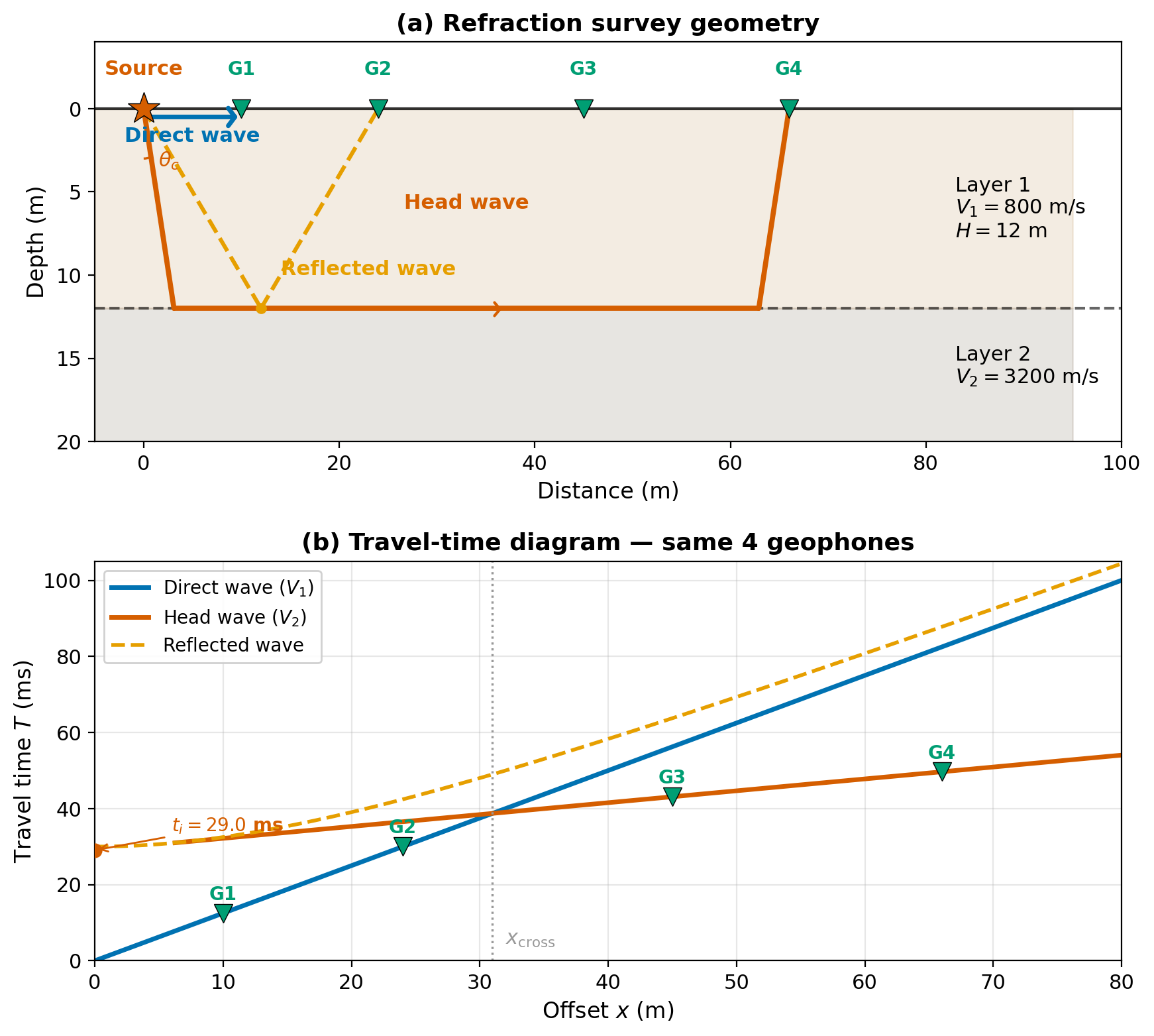— Fig. 20 **Figure 6.1.** Refraction survey geometry for a two-layer model. The direct wave travels at $V_1$ along the surface. The head wave descends at the critical angle $\theta_c$, travels along the interface at $V_2$, and returns to the surface at $\theta_c$. At close offsets the direct wave arrives first; beyond the crossover distance, the head wave arrives first. [Python-generated. Script: `assets/scripts/fig_refraction_survey_geometry.py`]#

2.2 Equipment (Brief)#

At the introductory scale, seismic refraction equipment is simple and portable. A sledgehammer striking a metal plate provides sufficient energy to detect interfaces down to ~30 m depth. The impact triggers a timing signal. An array of 12–48 geophones — small mechanical seismometers that convert ground velocity into electrical current via a coil-and-magnet system — is laid out at regular spacing (typically 2–5 m). A multichannel seismograph digitizes the output from all geophones simultaneously. For deeper targets (100s of meters to crustal scale), explosives, vibroseis trucks, or airguns replace the hammer, and 100s to 1000s of channels are deployed. Distributed Acoustic Sensing (DAS) — converting fiber-optic cables into continuous seismic arrays — is increasingly used for both shallow and deep refraction surveys.

3. Mathematical Framework#

3.1 Notation#

Notation

Symbol	Quantity	Units	Type
$V_1$	P-wave velocity in layer 1 (surface layer)	m/s	scalar
$V_2$	P-wave velocity in half-space (layer 2)	m/s	scalar
$H$	Thickness of layer 1	m	scalar
$x$	Source-receiver offset (horizontal distance)	m	scalar
$T(x)$	Travel time from source to receiver at offset $x$	s	scalar
$\theta_c$	Critical angle $= \arcsin(V_1/V_2)$	rad or °	scalar
$t_i$	Intercept time (head-wave $T$-axis intercept at $x=0$)	s	scalar
$x_\text{cross}$	Crossover distance (where head wave overtakes direct)	m	scalar
$p$	Ray parameter $= \sin\theta_c/V_1 = 1/V_2$	s/m	scalar

3.2 Direct Wave Travel Time#

The direct wave travels horizontally through layer 1 at velocity $V_1$. The travel time is simply distance divided by speed:

(53)#\[ T_\text{direct}(x) = \frac{x}{V_1} \]

This is a straight line through the origin with slope $1/V_1$. On a $T(x)$ plot, the slope of the direct-wave branch directly gives the reciprocal of the surface-layer velocity.

3.3 Head Wave Travel Time#

The head wave follows a three-segment path: (1) down from the surface to the interface at the critical angle $\theta_c$, (2) along the interface at speed $V_2$, and (3) back up to the surface at the critical angle.

Deriving the travel time: Consider a source at the surface and a receiver at offset $x$. The ray descends at angle $\theta_c$ from vertical through layer 1 of thickness $H$, reaching the interface at a horizontal distance $H\tan\theta_c$ from the source. It then travels horizontally along the interface for a distance $x - 2H\tan\theta_c$ (the middle segment), and ascends symmetrically to the receiver.

The travel time is the sum of three segments:

(54)#\[ T_\text{head}(x) = \underbrace{\frac{2H}{V_1\cos\theta_c}}_{\text{down + up in layer 1}} + \underbrace{\frac{x - 2H\tan\theta_c}{V_2}}_{\text{along interface}} \]

Expanding and using $\sin\theta_c = V_1/V_2$ and $\cos\theta_c = \sqrt{1 - V_1^2/V_2^2}$:

(55)#\[ T_\text{head}(x) = \frac{x}{V_2} + \frac{2H\cos\theta_c}{V_1} \]

Key Equation: Head Wave Travel Time

\[ T_\text{head}(x) = \frac{x}{V_2} + \frac{2H\cos\theta_c}{V_1} \]

This is a straight line with:

Slope $= 1/V_2$ — directly gives the velocity of the deeper layer
Intercept $t_i = 2H\cos\theta_c / V_1$ — encodes the layer thickness $H$

Units check: $[x/V_2] = \text{m}/(\text{m/s}) = \text{s}$. $[H\cos\theta_c/V_1] = \text{m}/(\text{m/s}) = \text{s}$ ✓

Derivation of the simplified form (intermediate steps):

Starting from (54):

\[ T = \frac{2H}{V_1\cos\theta_c} + \frac{x}{V_2} - \frac{2H\sin\theta_c}{V_2\cos\theta_c} \]

\[ = \frac{x}{V_2} + \frac{2H}{V_1\cos\theta_c}\left(1 - \frac{V_1\sin\theta_c}{V_2}\right) \]

Substituting $\sin\theta_c = V_1/V_2$:

\[ = \frac{x}{V_2} + \frac{2H}{V_1\cos\theta_c}\left(1 - \frac{V_1^2}{V_2^2}\right) = \frac{x}{V_2} + \frac{2H}{V_1\cos\theta_c}\cdot\cos^2\theta_c = \frac{x}{V_2} + \frac{2H\cos\theta_c}{V_1} \]

3.4 The Intercept Time#

The intercept time $t_i$ is the $T$-axis intercept of the head-wave line (extrapolated to $x = 0$):

(56)#\[ t_i = \frac{2H\cos\theta_c}{V_1} = \frac{2H\sqrt{V_2^2 - V_1^2}}{V_1 V_2} \]

Solving for the layer thickness:

(57)#\[ H = \frac{t_i V_1}{2\cos\theta_c} = \frac{t_i V_1 V_2}{2\sqrt{V_2^2 - V_1^2}} \]

Key Equation: Layer Depth from Intercept Time

\[ H = \frac{t_i\,V_1\,V_2}{2\sqrt{V_2^2 - V_1^2}} \]

Once $V_1$ (from the direct-wave slope) and $V_2$ (from the head-wave slope) are measured, the intercept time $t_i$ directly yields the layer thickness $H$.

3.5 The Critical Distance#

The head wave does not exist at arbitrarily small offsets. For a head wave to reach the surface, the ray must descend to the interface, travel some finite distance along it, and then return. The critical distance $x_\text{crit}$ is the minimum source-receiver offset at which a head wave can be observed.

From the geometry of the critical-angle ray path: the downgoing leg reaches the interface at a horizontal distance $H\tan\theta_c$ from the source, and the upgoing leg returns to the surface another $H\tan\theta_c$ away. Therefore:

(58)#\[ x_\text{crit} = 2H\tan\theta_c \]

For $x < x_\text{crit}$, head-wave arrivals are geometrically impossible — the region on the T(x) diagram below $x_\text{crit}$ is blank for the head-wave branch.

Critical Distance vs. Crossover Distance

Critical distance $x_\text{crit} = 2H\tan\theta_c$: minimum offset at which the head wave exists.
Crossover distance $x_\text{cross}$: offset at which the head wave becomes the first arrival, always satisfying $x_\text{cross} > x_\text{crit}$.

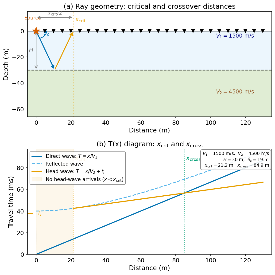
Two-panel figure. Top panel shows a two-layer cross-section with source at origin, geophones along the surface, and the critical-angle ray path descending to the interface and returning to the surface at the critical distance x_crit. Bottom panel shows T-x travel-time diagram with direct wave, head wave, intercept time t_i, and both x_crit and x_cross marked. — Fig. 21 **Figure 6.3.** Critical distance and crossover distance in a two-layer refraction model. The head wave is absent for x less than x_crit (shaded zone). The crossover occurs at the larger distance x_cross. [Python-generated. Script: assets/scripts/fig_refraction_critical_distance.py]#

3.6 How the T(x) Diagram Is Built: A Frame-by-Frame View#

A concrete way to understand the T(x) diagram is to watch it being constructed geophone by geophone as the wavefield propagates. At each receiver the first-arriving energy is recorded, and together these picks define the two linear branches.

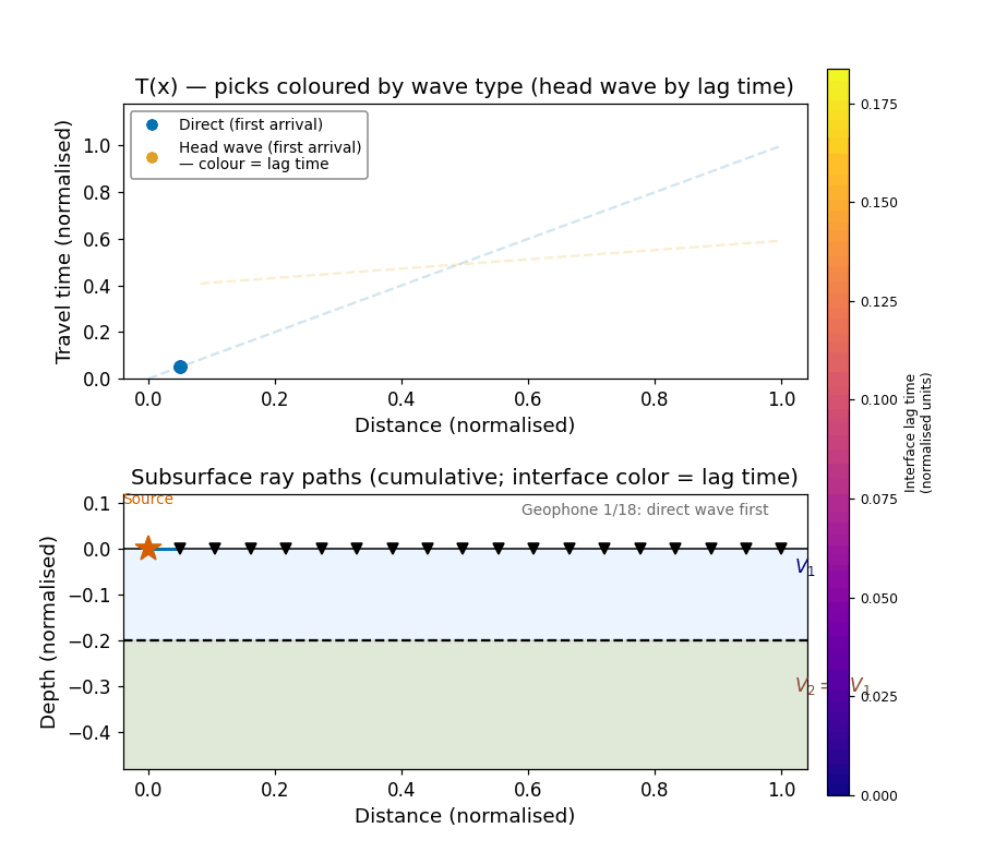
Animated refraction wavefield: geophone picks appear one by one on the T-x diagram as ray paths accumulate in the subsurface cross-section. Near-offset picks follow the direct-wave branch; far-offset picks follow the head-wave branch. Plasma color encodes interface lag time. — Fig. 22 **Figure 6.4.** Animated construction of the T(x) diagram — geophone picks appear one by one as ray paths accumulate. Near-offset picks (blue) follow the direct-wave branch; far-offset picks (plasma colors) follow the head-wave branch. The plasma color encodes the interface lag time. [Python-generated. Script: `assets/scripts/fig_refraction_wavefield_animation.py`]#

3.7 The Crossover Distance#

The crossover distance $x_\text{cross}$ is where the direct wave and head wave arrive at the same time:

\[ T_\text{direct}(x_\text{cross}) = T_\text{head}(x_\text{cross}) \]

\[ \frac{x_\text{cross}}{V_1} = \frac{x_\text{cross}}{V_2} + \frac{2H\cos\theta_c}{V_1} \]

Solving:

\[ x_\text{cross}\left(\frac{1}{V_1} - \frac{1}{V_2}\right) = \frac{2H\cos\theta_c}{V_1} \]

(59)#\[ x_\text{cross} = \frac{2H\cos\theta_c\,V_2}{V_2 - V_1} = 2H\sqrt{\frac{V_2 + V_1}{V_2 - V_1}} \]

Key Concept: The Crossover Distance

At $x < x_\text{cross}$, the direct wave arrives first (shorter path, slower speed wins). At $x > x_\text{cross}$, the head wave arrives first (longer path, but faster speed wins — the detour through the fast layer more than compensates for the extra distance). The crossover distance is always greater than the critical distance $x_\text{crit} = 2H\tan\theta_c$ (the minimum offset at which the head wave exists).

3.6 The Travel-Time Plot#

Travel-time plot with offset x on the horizontal axis and travel time T on the vertical axis. Three curves are shown. The direct wave is a straight line through the origin with slope 1 over V_1 in blue. The head wave is a straight line with shallower slope 1 over V_2 in green, offset upward by the intercept time t_i. The reflected wave is a hyperbola in orange starting at T_0 equals 2H over V_1 at x equals zero and approaching the direct wave asymptotically. The crossover distance x_cross where the direct and head wave lines intersect is marked with a vertical dashed line. The critical distance x_crit where the head wave first exists is also marked. For x less than x_cross the first arrival follows the direct wave; for x greater than x_cross the first arrival follows the head wave. 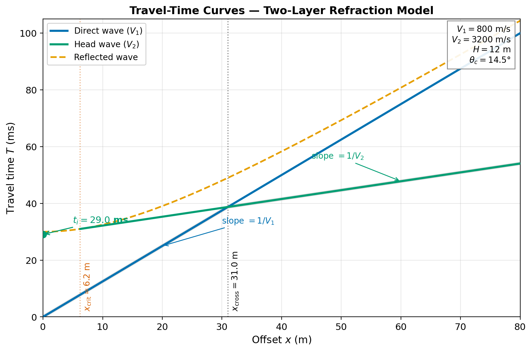— Fig. 23 **Figure 6.2.** Travel-time curves for a two-layer model. The first-arrival curve (bold) follows the direct wave at short offsets and the head wave at long offsets. The slopes give $V_1$ and $V_2$; the intercept time $t_i$ gives the layer depth $H$. The reflected wave (dashed) is a hyperbola — it is always slower than the first arrival and is the target of reflection surveys (Lectures 10–14). [Python-generated. Script: `assets/scripts/fig_refraction_travel_times.py`]#

4. The Forward Problem#

Given a two-layer model ($V_1$, $V_2$, $H$), the forward problem predicts the complete set of first-arrival travel times at every offset:

(60)#\[\begin{split} T_\text{first}(x) = \begin{cases} x/V_1 & \text{if } x \leq x_\text{cross} \\ x/V_2 + t_i & \text{if } x > x_\text{cross} \end{cases} \end{split}\]

See companion notebook: notebooks/Lab2-Python-Ray-Tracing.ipynb — students compute and plot these curves.

Worked Example — Shallow Refraction Survey on the UW Campus:

A refraction survey on the UW campus uses a sledgehammer source and 24 geophones at 3 m spacing (offsets 3–72 m). The subsurface consists of glacial till ($V_1 = 800$ m/s) over bedrock ($V_2 = 3200$ m/s) at depth $H = 12$ m.

Critical angle: $\theta_c = \arcsin(800/3200) = \arcsin(0.25) = 14.5°$

Intercept time: $t_i = 2 \times 12 \times \cos(14.5°) / 800 = 24 \times 0.968 / 800 = 0.0290$ s = 29.0 ms

Crossover distance: $x_\text{cross} = 2 \times 12\sqrt{(3200+800)/(3200-800)} = 24\sqrt{4000/2400} = 24 \times 1.291 = 31.0$ m

At geophone 10 ($x = 30$ m): direct wave arrives at $T = 30/800 = 37.5$ ms; head wave at $T = 30/3200 + 29.0 = 9.4 + 29.0 = 38.4$ ms. The direct wave is still faster — consistent with $x < x_\text{cross} = 31$ m.

At geophone 12 ($x = 36$ m): direct $T = 45.0$ ms; head wave $T = 11.3 + 29.0 = 40.3$ ms. The head wave now arrives first.

5. The Inverse Problem#

Inverse Problem: The Slope-Intercept Method

The refraction inverse problem is remarkably clean for a two-layer model:

Pick first arrivals on the shot gather — the time of the first P-wave motion at each geophone
Plot $T$ vs. $x$ — the first-arrival travel-time curve
Fit two straight-line segments:
- Near-offset slope = $1/V_1$ → $V_1$
- Far-offset slope = $1/V_2$ → $V_2$
Read the intercept time $t_i$ from the $T$-axis intercept of the head-wave line
Compute the layer depth: $H = t_i V_1 V_2 / (2\sqrt{V_2^2 - V_1^2})$

Non-uniqueness warning: This method assumes $V_2 > V_1$ (no velocity inversion), flat horizontal interfaces, and homogeneous layers. If a layer exists with $V_\text{hidden} < V_2$ between layers 1 and 2, it produces no head wave and is invisible — a hidden layer. Velocity inversions (slower layer beneath faster) are also invisible to first-arrival refraction. These limitations are addressed in Lecture 7.

6. Worked Example: Field Survey — Sledgehammer and Geophones#

The following example illustrates the full workflow from shot gather to subsurface model, replacing the copyrighted W.W. Norton Figs 3.6 and 3.7g with a fully reproducible synthetic equivalent that matches the same velocity contrasts.

A 13-geophone survey uses a sledgehammer source with receivers at 5–38 m spacing (3 m intervals). The subsurface model is dry sand ( \approx 350$ m/s) over saturated material ( \approx 1500$ m/s) — the classic water-table scenario.

Three-panel figure. Panel A shows a wiggle-trace shot gather with 13 horizontal traces, one per geophone at distances 5 to 38 m. Time increases to the right from 0 to 130 milliseconds. Each trace shows a Ricker-wavelet arrival with positive wiggles filled in blue. Red triangles mark the first-arrival picks. At near offsets the picks form a steep trend corresponding to the direct wave; at far offsets the picks show a shallower slope corresponding to the head wave. Panel B shows the raw first-arrival picks as dots on a time versus distance plot, with the knee visible near the crossover distance. Panel C shows the same picks with two best-fit lines: the direct-wave branch in blue with slope 1 over V_1 and the head-wave branch in orange with slope 1 over V_2. The intercept time t_i is marked on the time axis. A box gives the inversion result V_1 equals 350 m per s, V_2 equals 1500 m per s, H equals 5 metres. 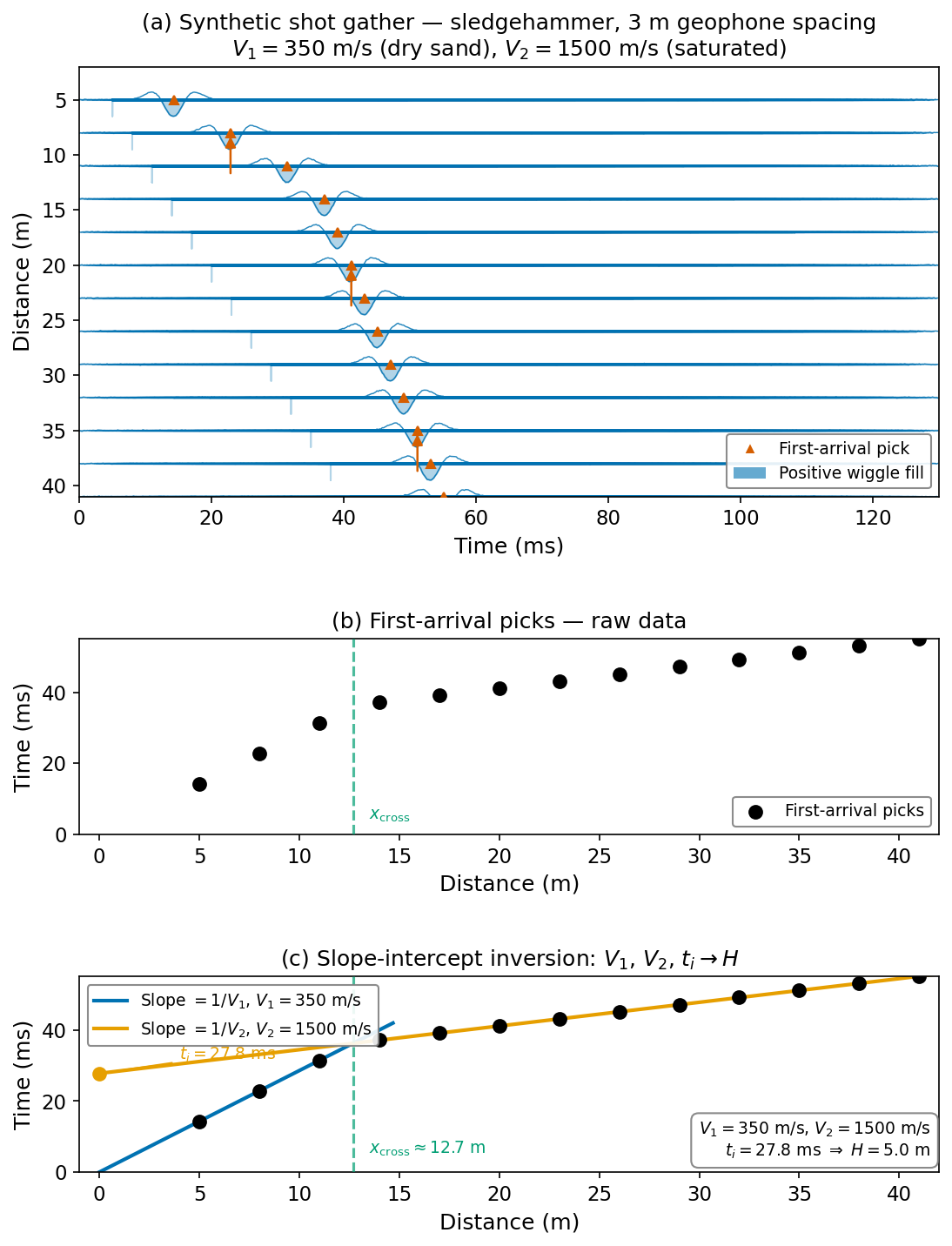— Fig. 24 **Figure 6.5.** Synthetic refraction field survey. (a) Shot gather: first arrivals (red triangles) shift from the steep direct-wave trend to the shallower head-wave trend beyond the crossover distance. (b) Raw first-arrival picks. (c) Slope-intercept inversion: two fitted lines give $, $, and \to H$. [Python-generated. Script: ]#

Reading the T(x) plot:

The “knee” in the first-arrival trend — the point where the steep direct-wave branch transitions to the shallower head-wave branch — occurs at the crossover distance \text{cross}$. In this model:

$ x_\text{cross} = 2 \times 5.0\sqrt{\frac{1500 + 350}{1500 - 350}} = 10\sqrt{\frac{1850}{1150}} \approx 12.7 \text{ m} $

The intercept time read from the far-offset line extrapolated to = 0$:

$ t_i = \frac{2 \times 5.0 \times \cos\theta_c}{350}, \quad \theta_c = \arcsin(350/1500) = 13.5° $

$ t_i = \frac{10 \times 0.972}{350} = 0.0278 \text{ s} = 27.8 \text{ ms} $

The depth to the water table:

$ H = \frac{t_i V_1 V_2}{2\sqrt{V_2^2 - V_1^2}} = \frac{0.0278 \times 350 \times 1500}{2\sqrt{1500^2 - 350^2}} = \frac{14595}{2 \times 1459} = 5.0 \text{ m} $

The inversion recovers the true layer depth exactly, as expected for noise-free synthetic data. Real field data introduces scatter in the picks (due to near-surface heterogeneity, instrument noise, and imperfect source coupling), so $ is estimated by least-squares line fitting rather than graphical reading.

7. Worked Example: Detecting the Water Table#

A shallow refraction survey measures:

Direct wave slope: $1/V_1 = 1/350$ s/m → $V_1 = 350$ m/s (dry sand above water table)
Head wave slope: $1/V_2 = 1/1500$ s/m → $V_2 = 1500$ m/s (saturated sand below water table)
Intercept time: $t_i = 0.012$ s

The water-table depth:

\[ \theta_c = \arcsin(350/1500) = \arcsin(0.233) = 13.5° \]

\[ H = \frac{0.012 \times 350}{2\cos(13.5°)} = \frac{4.20}{2 \times 0.972} = \frac{4.20}{1.945} = 2.16 \text{ m} \]

The water table is at 2.2 m depth. The dramatic velocity increase (350 → 1500 m/s) occurs because saturating sand pores with water increases the bulk modulus $K$ enormously (the incompressibility of water dominates) while the shear modulus $\mu$ remains nearly unchanged — exactly the $V_P/V_S$ physics from Lecture 4.

Concept Check

A two-layer model has $V_1 = 2000$ m/s, $V_2 = 5500$ m/s, $H = 50$ m. Calculate: (a) the critical angle, (b) the intercept time, (c) the crossover distance. At what geophone spacing would you need to place receivers to observe the crossover?
Explain in three sentences why the head wave — which travels a longer path than the direct wave — can arrive earlier at a distant receiver. Your explanation should reference both the fast-layer velocity and the geometry of the critical angle.
A travel-time plot shows a direct-wave slope of 5.0 ms/m and a head-wave slope of 1.25 ms/m with intercept $t_i = 30$ ms. Determine $V_1$, $V_2$, and $H$.
An AI assistant states: “The refraction method can detect all subsurface layers.” Critique this statement. Under what specific conditions does a layer become invisible to refraction?

8. Course Connections#

Prior lecture (Lecture 5): Snell’s law, the critical angle, and mode conversion — the physics that produces head waves — were derived in Lecture 5. This lecture applies those results to build a complete subsurface imaging method.
Next lecture (Lecture 7 — Seismic Refraction II): Extends to dipping layers (forward and reverse shooting), multiple layers, hidden layers, and velocity inversions.
Lectures 10–14 (Seismic Reflection): The reflected wave — the hyperbolic branch on the travel-time plot — is the target of reflection seismology. The refraction method sees the slopes (velocities); the reflection method sees the curvature (two-way travel time to interfaces).
Lab 2 (Apr 10): Students implement the direct-wave and head-wave travel-time equations in Python and compare to synthetic shot gathers.
Lab 3 (Apr 17): Students pick first arrivals on a real or synthetic refraction dataset and apply the slope-intercept inversion to determine $V_1$, $V_2$, and $H$.

9. Research Horizon#

Current Research Highlights (2022–2025)

DAS-based refraction surveys for shallow structure. Distributed Acoustic Sensing (DAS) is transforming refraction surveying. A single fiber-optic cable replaces hundreds of geophones, with channel spacing of 1–2 m over kilometers of profile. Ajo-Franklin et al. (2019, Scientific Reports, doi:10.1038/s41598-018-36675-8) demonstrated that dark-fiber DAS arrays in urban Sacramento detected refraction arrivals from shallow velocity contrasts invisible to conventional geophone arrays. The head-wave slopes on the DAS shot gathers are interpreted using exactly the equations from §3.3 — but with orders-of-magnitude more spatial sampling.

Ambient noise refraction. Classical refraction requires an active source. Emerging methods extract refraction-like arrivals from ambient seismic noise correlations, enabling passive refraction surveys in environments where active sources are impractical (urban areas, environmentally sensitive sites). Nakata et al. (2015, Geophysics, doi:10.1190/geo2014-0223.1) showed that noise-based body wave retrieval recovers head-wave arrivals consistent with active-source results.

Machine learning first-break picking. The rate-limiting step in refraction processing is picking the first arrival on each trace. Deep-learning models trained on thousands of labeled shot gathers now automate this step with sub-millisecond precision, dramatically accelerating the workflow from field data to velocity model (Yuan et al., 2023, Geophysics, doi:10.1190/geo2022-0286.1 (⚠ DOI returns 404 — verify manually)).

Student entry point: The IRIS “Determining Shallow Earth Structure” activity (CC BY) provides real refraction data for classroom inversion: iris.edu/hq/inclass/lesson/determining_shallow_earth_structure.

10. Societal Relevance#

Why It Matters: Shallow Refraction for Infrastructure and Hazard

Depth to bedrock for foundation design. Before constructing a bridge, tunnel, or high-rise, engineers need to know where bedrock is. A shallow seismic refraction survey determines bedrock depth in hours at a cost of a few thousand dollars — far cheaper and faster than drilling. The Sound Transit light rail extension in Seattle used refraction surveys to map the depth to glacial till and bedrock along proposed tunnel alignments, directly informing the choice between bored tunnels and cut-and-cover construction.

Water table detection. The dramatic P-wave velocity increase at the water table (from ~200–400 m/s in dry sand to ~1500 m/s in saturated sand) produces one of the strongest refraction signals in near-surface geophysics. Environmental site assessments routinely use refraction to map water-table depth without drilling, critical for contamination plume monitoring and groundwater resource management.

Crustal thickness from earthquake refraction. Mohorovičić’s 1909 method — using earthquake sources instead of hammers — remains the primary way to determine crustal thickness worldwide. The Moho depth beneath the Pacific Northwest varies from ~10 km under the ocean to ~40 km under the Cascades, and this variation is mapped entirely from refraction arrivals on regional seismograms recorded by the PNSN and EarthScope Transportable Array.

For further exploration:

IRIS Determining Shallow Earth Structure: iris.edu/hq/inclass/lesson/determining_shallow_earth_structure
USGS Crustal Structure of the US: earthquake.usgs.gov/data/crust
PNSN Cascadia velocity models: pnsn.org

AI Literacy#

AI as a Reasoning Partner: Checking the Travel-Time Derivation

The head-wave travel-time derivation (§3.3) involves three path segments, trigonometric substitutions, and a simplification that is easy to get wrong. This is a productive exercise for AI-assisted verification.

Prompt to try:

“Derive the head-wave travel time for a two-layer model. The surface layer has velocity V_1 and thickness H. The half-space has velocity V_2 > V_1. The ray descends at the critical angle theta_c, travels along the interface, and ascends at theta_c. Show every intermediate step and simplify to T = x/V_2 + 2Hcos(theta_c)/V_1.”*

Evaluate:

Does the AI correctly identify the three path segments?
Does it use $\sin\theta_c = V_1/V_2$ in the simplification?
Common error: writing $2H/V_1\cos\theta_c$ instead of $2H\cos\theta_c/V_1$ — these are very different! The correct form has $\cos\theta_c$ in the numerator.

AI Prompt Lab

Prompt 1:

“A refraction travel-time plot has a near-offset slope of 2.5 ms/m and a far-offset slope of 0.8 ms/m. The intercept time is 15 ms. Calculate V_1, V_2, and the depth to the interface.”

Evaluate: $V_1 = 400$ m/s, $V_2 = 1250$ m/s, $\theta_c = 18.7°$, $H = 3.3$ m. Check the AI’s arithmetic carefully — unit conversion errors (ms vs. s) are common.

Prompt 2:

“Can the refraction method detect a low-velocity layer sandwiched between two high-velocity layers? Explain physically why or why not.”

Evaluate: A low-velocity layer produces no head wave (no critical refraction from above) and is therefore invisible to first-arrival refraction. Does the AI explain the physics (no critical angle exists when $V_2 < V_1$) or just state the result?

References#

@book{lowrie2020,
  author    = {Lowrie, W. and Fichtner, A.},
  title     = {Fundamentals of Geophysics},
  edition   = {3rd},
  publisher = {Cambridge University Press},
  year      = {2020},
  doi       = {10.1017/9781108685917}
}

@misc{mitocw12510_lec6,
  title  = {12.510 Introduction to Seismology, Lecture 6: Travel-time curves},
  year   = {2010},
  note   = {MIT OpenCourseWare, CC BY NC SA},
  url    = {https://ocw.mit.edu/courses/12-510-introduction-to-seismology-spring-2010}
}

@article{ajofranklin2019,
  author  = {Ajo-Franklin, J. B. and others},
  title   = {Distributed Acoustic Sensing Using Dark Fiber for Near-Surface Characterization},
  journal = {Scientific Reports},
  volume  = {9},
  pages   = {1328},
  year    = {2019},
  doi     = {10.1038/s41598-018-36675-8}
}


Course LOs addressed	LO-1 (head waves as observables from velocity contrasts), LO-2 (travel-time equations as forward models), LO-3 (slope-intercept inversion for \(V_1\), \(V_2\), \(H\)), LO-4 (assumptions: flat layers, constant velocity, first arrivals only)
Learning outcomes practiced	LO-OUT-A (sketch refraction survey geometry), LO-OUT-B (compute head wave travel times, intercept times, crossover distances), LO-OUT-C (explain why head waves overtake direct waves), LO-OUT-D (set up the refraction inverse problem), LO-OUT-E (discuss non-uniqueness: hidden layers, velocity inversions)
Lowrie & Fichtner chapter	Ch. 6, §6.3.2–6.3.3 (free via UW Libraries)
Prior lecture	Lecture 5 — Wavefronts, Rays, and Waves at Boundaries (Snell’s law, critical angle, mode conversion)
Next lecture	Lecture 7 — Seismic Refraction II (dipping layers, multiple layers, hidden layers)
Lab connection	Lab 2 (Apr 10): Python II and Seismic Ray Tracing; Lab 3 (Apr 17): Refraction