Putting It Together: Geophysics as a Tool for Earth Structure

Putting It Together: Geophysics as a Tool for Earth Structure#

Learning Objectives

By the end of this lecture, students will be able to:

[LO-1 / LO-OUT-F] Explain why no single geophysical observable determines Earth structure uniquely, and how independent observables sensing different physical properties are combined to constrain one self-consistent Earth model.
[LO-3 / LO-OUT-D] Express the relationship between a single Earth model and several data types as a set of forward operators, and state the joint inverse problem that links them.
[LO-3 / LO-OUT-E] Use the oceanic lithosphere cooling model to show how one thermal model predicts both heat flow and seafloor subsidence, and interpret the misfit that signals when a model has reached its limit.
[LO-2 / LO-OUT-C] Estimate, using the Rayleigh number, why heat escapes the mantle by convection rather than conduction, and explain how plate tectonics and hotspots are the two surface expressions of that convection.
[LO-4] Identify the present frontiers of geophysics — machine learning, sensing technology, the cryosphere and environment, and planetary interiors — and the methodological reasons each is advancing now.
[LO-7 / LO-OUT-H] Evaluate an AI-generated synthesis of a multi-method geophysical argument against an explicit rubric, and document where the reasoning is sound, unsupported, or wrong.

Syllabus Alignment


Course LOs addressed	LO-1, LO-3, LO-4, LO-7
Learning outcomes practiced	LO-OUT-D, LO-OUT-E, LO-OUT-F, LO-OUT-H
Prior lecture	L29 — Transform & Intraplate Processes
Next lecture	Student Presentations / Course Wrap-Up
Lab connection	Lab AI — AI as a Geophysics Collaborator (rubric-driven evaluation)
Companion notebook	`notebooks/synthesis_joint_interpretation.ipynb`

Prerequisites#

This lecture draws on every module of the course. Familiarity with the following is assumed: seismic travel times and the velocity–structure relationship (Modules 1–3); the gravity anomaly and isostasy (Module 4); the magnetic anomaly and seafloor spreading (Module 5); and the conductive cooling of oceanic lithosphere (Module 7). The recurring theme of non-uniqueness, introduced with seismic refraction and revisited in tomography and potential-field interpretation, is the conceptual backbone here.

1. The Geoscientific Question#

Across ten weeks the course has assembled a toolkit: seismic refraction and reflection, whole-Earth and travel-time tomography, earthquake location and ground motion, gravity and isostasy, magnetics and plate kinematics, and the thermal evolution of the lithosphere. Each method was presented as a way to convert a surface measurement into a statement about the inaccessible interior. Each was also shown to be limited: a refraction survey cannot see beneath a low-velocity layer; a gravity anomaly is consistent with infinitely many density distributions; a single seismogram constrains a velocity model only weakly.

A practical question follows from this accumulation. Confronted with a real Earth structure — a subduction zone, a sedimentary basin, a stretch of oceanic lithosphere — which method should be applied, and how should the results of several methods be reconciled when each is individually ambiguous? The answer is the organizing idea of geophysics as a discipline, and the subject of this final lecture: independent observables, each sensitive to a different physical property of the same Earth, are far more powerful in combination than in isolation. The non-uniqueness of any one method is reduced when a model is required to explain all of them at once.

This lecture makes that idea quantitative using the best-constrained natural laboratory in the course — the cooling oceanic lithosphere — and then turns to the directions in which the discipline is now expanding.

2. Governing Physics#

The unifying observation is that the diverse geophysical measurements of the course are all functionals of a single underlying Earth model. A region of the Earth can be described by a model \(m\) collecting its geometry and its material and thermal properties: density \(\rho\), seismic velocities \(V_P\) and \(V_S\), temperature \(T\), magnetization, and rheology. Each measurement type is produced from that same \(m\) by a different piece of physics:

The elastic wave equation maps the velocity and density structure to seismic travel times and waveforms.
Newtonian gravity (the Poisson equation for the gravitational potential) maps the density structure to the gravity anomaly \(\Delta g\).
The magnetic potential field maps the magnetization — itself dependent on temperature through the Curie point — to the magnetic anomaly \(\Delta B\).
Fourier heat conduction maps the temperature field to the surface heat flow \(q\).
Elastic flexure and viscous flow, observed geodetically, map the lithospheric rheology to surface displacement measured by GPS and InSAR.

Important

Key Concept — one model, many sensitivities. Different methods do not measure different Earths; they measure different properties of the same Earth. Seismic velocity, density, temperature, and magnetization are physically linked (for example, hotter rock is generally slower and less dense). A model that satisfies the seismic data but predicts the wrong gravity is not a valid model of the region. Consistency across independent observables is the strongest available test of an Earth model.

This structure is shown schematically in Fig. 161: a single model on the left, fanned out through the forward operators of the course to the observables on the right, and closed by the joint inverse problem along the bottom.

A flow diagram. A single tall box on the left labeled "ONE Earth model m" lists geometry, density, P- and S-wave velocity, temperature, and magnetization. Five arrows fan out to five forward-operator boxes in the middle column — elastic wave equation, Newtonian gravity, magnetic potential field, Fourier heat conduction, and flexure and geodesy — each labeled with the property it senses. Each forward operator points to an observable box on the right: seismic travel times and waveforms, gravity anomaly, magnetic anomaly, surface heat flow, and GPS or InSAR displacement. A dashed return arrow along the bottom is labeled "joint inverse problem: find one m that explains all data at once," with the note that combining independent observables reduces non-uniqueness. 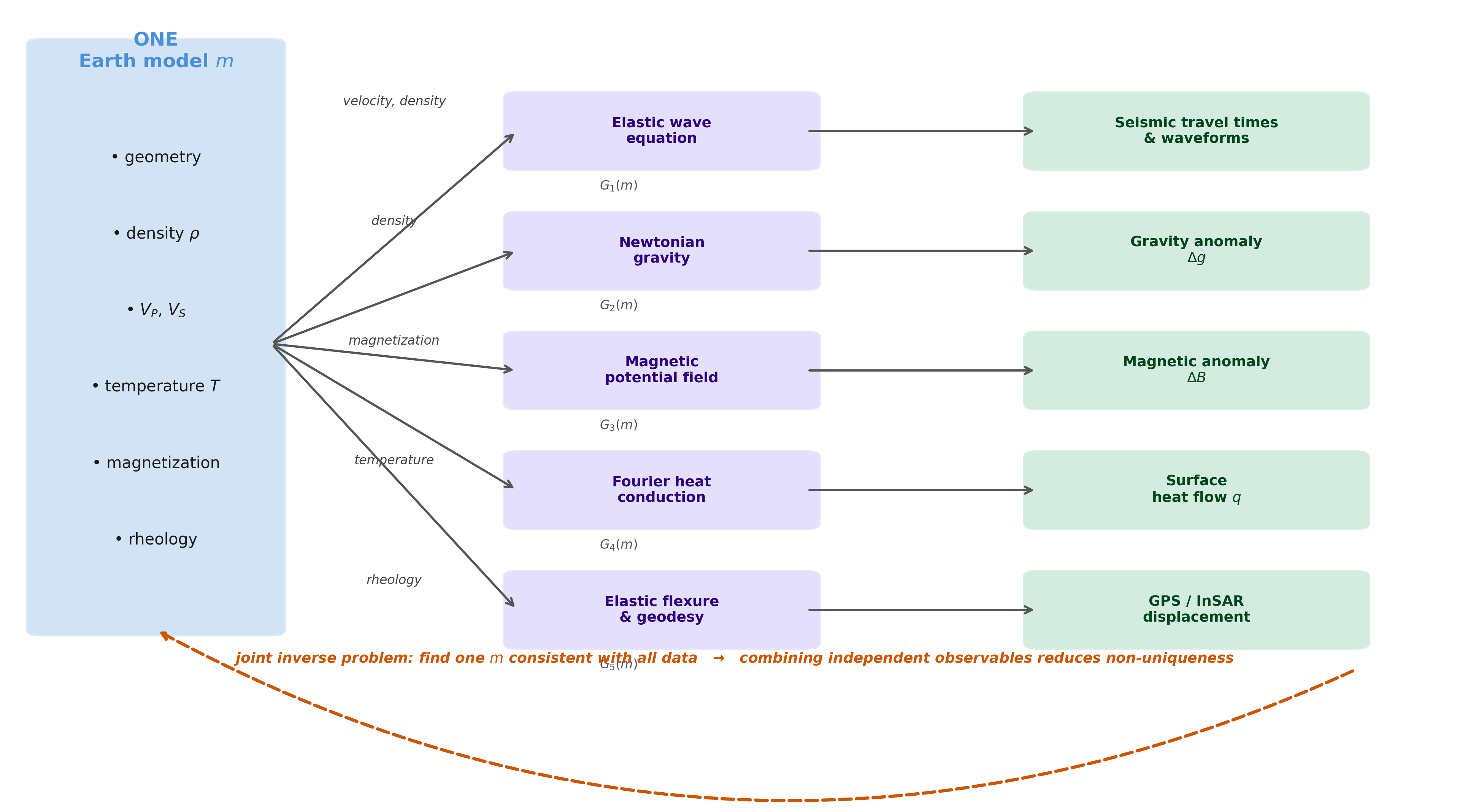— Fig. 161 One Earth model, many observables. Each forward operator \(G_i\) is a piece of physics taught earlier in the course; each maps the same model \(m\) to a different data type. The joint inverse problem requires a single \(m\) consistent with all of them.#

A second organizing idea sits beneath the first. The Earth model \(m\) is not static: the planet is cooling, and that cooling sets much of what the observables record. Heat flow measures it directly; the deepening of the seafloor records the cooling of one plate; the density and magnetization structure carry the thermal state. The synthesis therefore operates at two scales. At the local scale, a single oceanic plate cools as it ages — the worked example of sections 3–4. At the global scale, the whole planet cools, and the dominant way it sheds that heat — mantle convection — is the engine that drives plate tectonics and produces hotspots (section 3e and section 5). The local cooling model is one cold piece of the global convecting system.

Important

Key Concept — cooling at two scales. The half-space cooling of an oceanic plate (\(q \propto t^{-1/2}\)) is the cold upper thermal boundary layer of a mantle that is convecting as a whole. The same thermal physics that deepens the seafloor with age governs how the entire planet loses heat. Plate tectonics is the surface signature of that convection; hotspots are a second, independent signature that the rigid-plate picture alone cannot explain.

3. Mathematical Framework#

Notation

Symbol	Meaning	Units
\(m\)	Earth model (vector of parameters)	mixed
\(d_i\)	observation of type \(i\)	varies
\(G_i\)	forward operator for data type \(i\)	—
\(e_i\)	observational error in \(d_i\)	varies
\(\sigma_i\)	standard deviation of \(e_i\)	varies
\(T(z,t)\)	temperature at depth \(z\), seafloor age \(t\)	\(^\circ\mathrm{C}\)
\(T_m\)	mantle (asthenosphere) temperature	\(^\circ\mathrm{C}\)
\(T_s\)	seafloor surface temperature	\(^\circ\mathrm{C}\)
\(\kappa\)	thermal diffusivity	\(\mathrm{m^2\,s^{-1}}\)
\(k\)	thermal conductivity	\(\mathrm{W\,m^{-1}\,K^{-1}}\)
\(q(t)\)	conductive surface heat flow	\(\mathrm{mW\,m^{-2}}\)
\(d(t)\)	seafloor depth below ridge crest	\(\mathrm{m}\)
\(\rho_m,\ \rho_w\)	mantle, seawater density	\(\mathrm{kg\,m^{-3}}\)
\(\alpha\)	volumetric thermal expansivity	\(\mathrm{K^{-1}}\)

3a. The joint inverse problem#

Each observation type is related to the model by its forward operator, with additive error:

(210)#\[d_i = G_i(m) + e_i, \qquad i = 1, 2, \ldots, N .\]

A model is judged by how well it reproduces all of the data simultaneously. Assuming independent Gaussian errors, the combined misfit is

(211)#\[\chi^2(m) = \sum_{i=1}^{N} \frac{\bigl\lVert d_i - G_i(m) \bigr\rVert^2}{\sigma_i^2} .\]

The joint inverse problem is to find the model \(m\) that minimizes (211). The essential point is geometric: each data type alone leaves a null space — a set of model changes it cannot detect. Where the null spaces of two independent data types do not coincide, requiring both to be fit removes models that either alone would have permitted. Combining observables shrinks the null space; this is why joint interpretation reduces non-uniqueness rather than merely averaging it.

3b. A concrete case: one thermal model, two observables#

The oceanic lithosphere provides the cleanest natural example, because a single thermal model predicts two independent geophysical observables. Treating the cooling lithosphere as a half-space whose surface is held at \(T_s\) while its interior begins at \(T_m\), conductive cooling gives the temperature field

(212)#\[T(z,t) = T_s + (T_m - T_s)\,\operatorname{erf}\!\left( \frac{z}{2\sqrt{\kappa t}} \right),\]

where \(\operatorname{erf}\) is the error function and \(t\) is the age of the seafloor (the time since the lithosphere formed at the ridge). Equation (212) is the single model \(m\) for this region. Two distinct measurements follow from it.

The thermal observable. The surface heat flow is the conductive flux at \(z = 0\), \(q = -k\,\partial T/\partial z|_{z=0}\). Differentiating (212),

(213)#\[q(t) = \frac{k\,(T_m - T_s)}{\sqrt{\pi \kappa t}} \;\propto\; t^{-1/2} .\]

The density observable. As the lithosphere cools it contracts and becomes denser; isostatic balance then requires the seafloor to deepen with age. Integrating the thermal contraction of the column and applying isostasy gives

(214)#\[d(t) = d_r + \frac{2\,\rho_m\,\alpha\,(T_m - T_s)}{\rho_m - \rho_w}\sqrt{\frac{\kappa t}{\pi}} \;\propto\; t^{1/2},\]

where \(d_r\) is the ridge-crest depth. Heat flow is read through a thermal measurement; seafloor depth is read through bathymetry and the gravity field. They are independent observations — yet both are fixed by the same \(T(z,t)\).

Key Equation

Heat flow falls as the inverse square root of age, (213), while seafloor depth grows as the square root of age, (214). The same three quantities — \((T_m - T_s)\), \(\kappa\), and the material constants — control both. A thermal model that fits the heat flow but not the bathymetry, or the reverse, is rejected. This is the joint inverse problem in its simplest non-trivial form.

The age \(t\) in equations (213) and (214) is not itself measured thermally — it is read from the magnetic anomaly pattern of the seafloor. The paleomagnetic reversal stripes recorded symmetrically about the ridge crest (L23–L25) identify the age of each strip of lithosphere with precision and serve as the direct input to the thermal equations. The plate-cooling synthesis therefore spans three independent observing systems — magnetics (age), heat-flow probes (thermal flux), and bathymetry (depth) — each measuring a different physical property of the same lithosphere, all constraining the same thermal parameters. Over young seafloor, measured heat flow falls systematically below the half-space prediction because hydrothermal circulation carries heat advectively through the porous young crust; the mismatch between the magnetically determined age-prediction and the measured heat flow localizes zones of active hydrothermal recharge.

3c. Seismic velocity and gravity: joint crustal imaging#

Seismic P-wave velocity and bulk density are physically related: in crustal and upper-mantle rocks they follow the empirical Nafe\u2013Drake curve, where denser rocks propagate P waves faster across a wide range of compositions. This link is the physical bridge between the elastic-wave forward operator (L03\u2013L13) and the Newtonian gravity forward operator (L19\u2013L22) — the two most prevalent method families in the course.

A refraction or wide-angle reflection survey produces a \(V_P\) model of the crust. Converting each cell to a density through the Nafe\u2013Drake relation generates a predicted Bouguer or free-air anomaly that can be compared with the observed field. Where prediction matches observation, the velocity model is a self-consistent description of the density structure. Where they disagree, the gravity residual localizes compositional anomalies — serpentinized mantle, mafic intrusions, evaporite bodies — that are either invisible to seismic refraction or too subtle in velocity contrast to resolve clearly.

The benefit flows in both directions. Gravity inversion alone suffers from the equivalent-source ambiguity introduced in L19\u2013L20: infinitely many depth\u2013density combinations produce an identical surface anomaly. Coupling the gravity inversion to a seismic \(V_P\) model removes that ambiguity for the resolved structures, shrinking the null space of (211) in exactly the sense of section 3a. The joint result — crustal thickness, slab geometry, wedge density — is more constrained than either observable alone.

3d. Earthquake source, strong motion, and hazard: a multi-observable synthesis#

Seismic hazard assessment is the course’s most consequential synthesis problem: it draws on more observing systems than any other application in ESS 314. Estimating what an earthquake will do to a site requires at least four independent data streams, each sensing a different aspect of the same fault.

Fault geometry from seismic imaging. Reflection and refraction surveys constrain fault-plane geometry and the \(V_P\) model used to locate earthquakes; local seismicity traces the Wadati\u2013Benioff zone; teleseismic tomography images the slab and identifies where the seismogenic zone is widest (L11\u2013L13, L28). The seismogenic width \(W\) in \(M_0 = \mu\,\bar{D}\,L\,W\) is controlled by the brittle\u2013ductile transition depth — itself a thermal quantity, connecting the hazard problem to sections 3b and 3e.

Past rupture from waveform inversion. Fitting seismogram waveforms to recover the moment tensor and \(M_0\) is an instance of (211) with the elastic wave equation as the forward operator and the double-couple source parameters as the model (L14\u2013L16). For historical events, long-period surface waves and geodetic co-seismic offsets provide independent data types for the same inversion.

Present-day loading from geodesy. GPS and InSAR map the interseismic surface velocity field; inverting for slip deficit on the fault (structurally identical to (211)) gives the spatial coupling distribution — where elastic strain is accumulating to be released in the next rupture. At Cascadia, this geodetic inversion predicts which segments will participate in the next \(M\,9\) event.

Future shaking and tsunami from forward modeling. Ground-motion prediction equations translate \(M_w\), source\u2013site distance, and site \(V_{s30}\) into engineering shaking intensity (L17). Tsunami generation and propagation use the same fault-slip distribution as the sea-surface initial condition (L18). A complete hazard model satisfies the seismic imaging, the geodetic coupling, the paleoseismic record, and ground-motion observations from past earthquakes simultaneously — one consistent fault model explaining all observables, exactly the logic of Fig. 161.

3e. From a cooling plate to a cooling planet#

The plate of section 3b cools because it loses heat to the ocean above. The whole Earth does the same on a far larger scale. Summed over its surface, the planet loses heat at a rate of approximately \(46\ \mathrm{TW}\) [Davies and Davies, 2010]. About half of this is replaced by the radioactive decay of uranium, thorium, and potassium distributed through the mantle and crust; the remainder is secular cooling — heat left over from accretion and core formation, released as the planet slowly cools, together with a contribution of roughly \(5\text{–}15\ \mathrm{TW}\) conducted out of the core across the core–mantle boundary. The Earth is, in the most literal sense, a cooling body, and the question is how that heat escapes.

Heat can leave by conduction alone, or the material can move and carry heat with it by convection. Which mechanism dominates is decided by a single dimensionless number — the Rayleigh number — that compares the vigour of buoyancy-driven flow with the damping effects of viscosity and thermal diffusion:

(215)#\[Ra = \frac{\rho\, g\, \alpha\, \Delta T\, D^{3}}{\kappa\, \eta},\]

where \(g\) is gravitational acceleration, \(\Delta T\) the temperature contrast across a layer of thickness \(D\), and \(\eta\) the dynamic viscosity (the other symbols as in the notation table). When \(Ra\) exceeds a critical value of order \(10^{3}\), small thermal perturbations grow into organized flow and convection sets in.

Key Equation

For the mantle — a layer roughly \(D \approx 2.9\times10^{6}\ \mathrm{m}\) thick with a temperature contrast of order \(10^{3}\ \mathrm{K}\) and a viscosity near \(10^{21}\ \mathrm{Pa\,s}\) — equation (215) gives \(Ra \sim 10^{6}\text{–}10^{8}\), far above critical. The mantle convects: it sheds the planet’s heat by flowing, not by conduction. A pot of water on a stove reaches a high Rayleigh number for the same reason and convects visibly; the mantle does the same, immeasurably more slowly. The conduction-only cooling of section 3b is therefore valid only in the cold upper boundary layer — the lithosphere — where the rock is too stiff to flow. Below it, heat moves by convection.

This convection is not an abstraction: its limbs are observable at the surface. Cold, dense lithosphere sinks as subducting slabs (downwellings); hot material rises beneath ridges (passive, shallow upwelling) and in narrow plumes from the deep mantle (active upwelling). Fig. 162 in section 5 shows the planform, and section 5 connects it to plate tectonics and to hotspots.

4. Worked Example#

Consider a site on 50-million-year-old oceanic seafloor. Using the numerical forms from section 3:

Heat flow: \(q = 510 / \sqrt{50} = 510 / 7.07 \approx 72\ \mathrm{mW\,m^{-2}}\).
Seafloor depth: \(d = 2500 + 350\sqrt{50} = 2500 + 2475 \approx 4975\ \mathrm{m}\).

Both predictions come from the same model. A measured heat flow near \(72\ \mathrm{mW\,m^{-2}}\) and a measured depth near \(5000\ \mathrm{m}\) would jointly confirm the cooling model at this age; a mismatch in either would demand revision.

Seismic moment and fault dimensions. The Cascadia megathrust has well-constrained geometry: \(L \approx 1000\ \mathrm{km}\) along strike and \(W \approx 100\ \mathrm{km}\) downdip. Paleoseismic evidence (drowned coastal forests and Japanese tsunami records) fixes average coseismic slip in the 1700 rupture at \(\bar{D} \approx 15\ \mathrm{m}\). Using \(\mu = 30\ \mathrm{GPa}\) for the shallow megathrust:

\[M_0 = \mu\,\bar{D}\,L\,W = 3\times10^{10}\ \mathrm{Pa} \times 15\ \mathrm{m} \times 10^{6}\ \mathrm{m} \times 10^{5}\ \mathrm{m} = 4.5\times10^{22}\ \mathrm{N\cdot m},\]

\[M_w = \tfrac{2}{3}\log_{10}(4.5\times10^{22}) - 6.07 \approx 9.0.\]

Three forward operators then act on this single source model. The elastic wave equation predicts teleseismic waveform amplitudes, consistent with the magnitude inferred independently from Japanese tsunami records. A ground-motion prediction equation (L17) maps \(M_w\) and source\u2013site distance to expected shaking intensity along the I-5 corridor. The shallow-water wave equation (L18) propagates the fault-slip sea-surface deformation to predict run-up heights along the coast. All three use the same \(M_0\) and fault geometry — three independent physical predictions from one source model, each testable against separate observations.

5. Connecting to Cascadia: From Local Cooling to the Global Engine#

This lecture is deliberately a return visit to the whole course. The forward operators in Fig. 161 are, in order, the subjects of Modules 1–3 (the elastic wave equation and seismic imaging), Module 4 (gravity and isostasy), Module 5 (magnetics and the magnetization–temperature link through the Curie point), and Module 7 (the thermal lithosphere and flexure). The non-uniqueness argument formalizes a thread that began with the hidden-layer problem in seismic refraction, recurred in the equivalent-source ambiguity of potential fields, and was named explicitly in tomography. The plate-cooling spine ties Module 7’s thermal model to Module 4’s isostasy and to the seafloor ages read from Module 5’s magnetic stripes — three modules in one model.

The cooling of one plate (section 3b) and the cooling of the whole planet (section 3e) are the same physics at two scales. The convecting mantle that sheds the Earth’s heat (Fig. 162) presents itself at the surface in two ways. Its cold, organized downwellings are the subducting slabs of plate tectonics; its passive shallow upwellings rise beneath the mid-ocean ridges. Plate tectonics, in this light, is the surface expression of mantle convection — the cold upper boundary layer of the convecting system, broken into plates that diverge where material rises and converge where it sinks.

A cross-section of the mantle from the surface to the core-mantle boundary at 2890 kilometres depth, with the liquid iron outer core shown below. At the surface, a mid-ocean ridge has diverging arrows above a shallow passive upwelling, and a hotspot volcano sits above a narrow plume. A blue subducting slab descends from a trench on the right as a cold dense downwelling, with downward arrows. A vermilion plume rises from a hot D-double-prime thermal boundary layer at the core-mantle boundary toward the hotspot; near the top the plume is bent sideways by a green horizontal arrow labelled mantle wind. A boxed Rayleigh number formula notes that the mantle Rayleigh number of ten-to-the-six through ten-to-the-eight greatly exceeds the critical value near ten-to-the-three, so the mantle convects and moves heat by flow rather than conduction. Orange arrows mark surface heat loss of about 46 terawatts and heat from the core of about 5 to 15 terawatts. 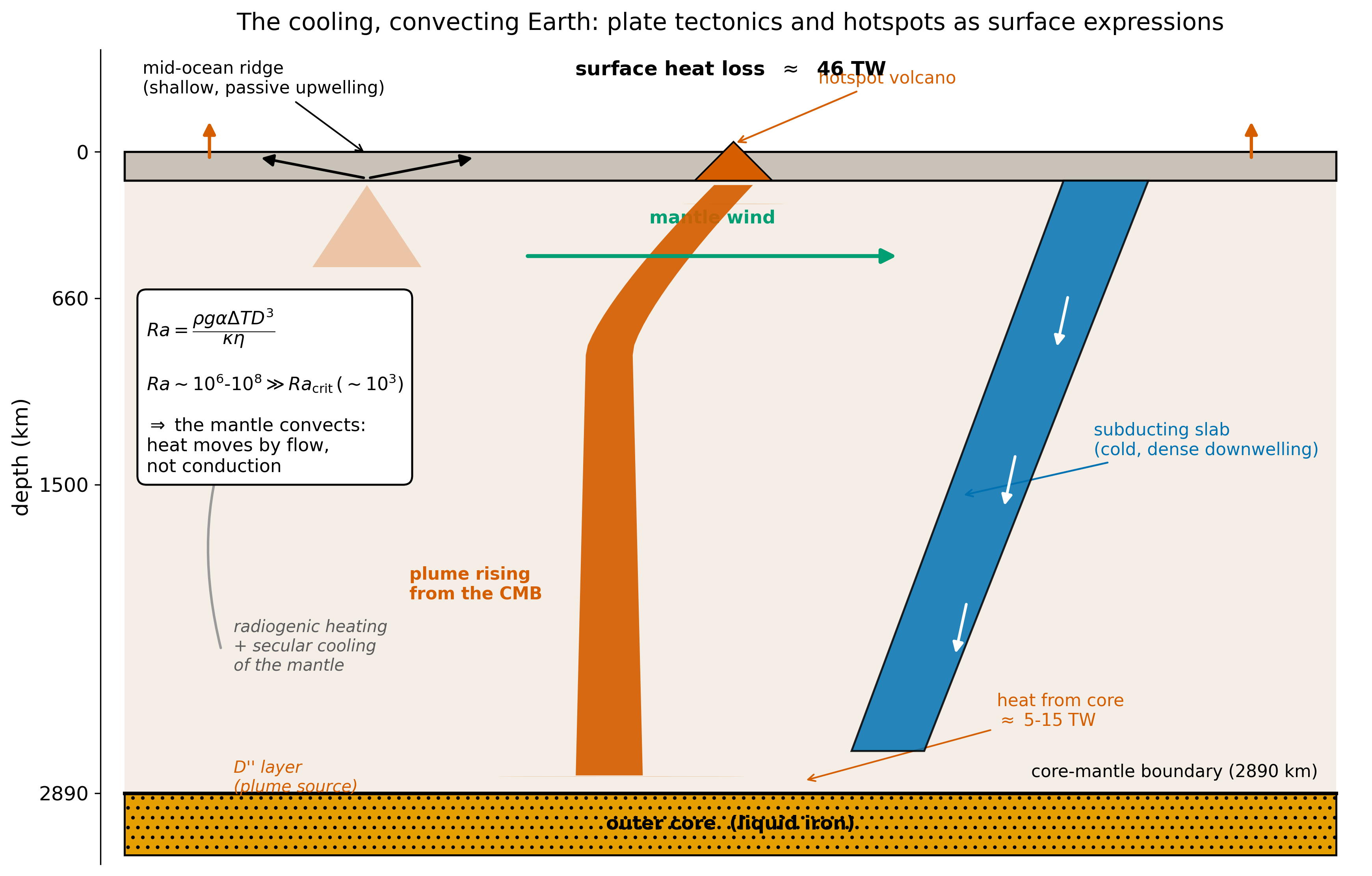— Fig. 162 The cooling, convecting Earth. The mantle’s high Rayleigh number means it sheds heat by convection. Plate tectonics is the cold downwelling-and-divergence limb at the surface; hotspots are the hot upwelling limb, rising as narrow plumes from the core–mantle boundary and bent by large-scale mantle flow.#

Hotspots: where the rigid-plate picture breaks#

Plate tectonics describes the surface as a mosaic of rigid plates whose relative motions are concentrated at their boundaries. It is a kinematic description — it states how plates move, not what drives them — and it works remarkably well. Hotspots are where that clean picture breaks, and the break is informative.

The first disruption is location. Volcanic chains such as Hawai’i–Emperor erupt in plate interiors, thousands of kilometres from any plate boundary, where the rigid-plate paradigm provides no mechanism for melting. Their age-progressive tracks are most simply explained by a melting source fixed in the deeper mantle, over which the plate slides — so the track records the plate’s absolute motion and direction. The source is a mantle plume, and seismic imaging now traces many plumes to the lowermost mantle, rooted near the margins of the large low-shear-velocity provinces above the core–mantle boundary [Koppers et al., 2021].

The second disruption is fixity. The hotspot reference frame was long treated as the absolute frame for plate motion, on the assumption that plumes are anchored rigidly at depth. They are not. Because plumes rise slowly through a mantle that is itself flowing, they are bent and dragged sideways by that large-scale flow — a “mantle wind” (Fig. 162). A deflected plume produces a hotspot that migrates over geologic time, so the frame is only approximately fixed; correcting for plume motion is now part of any careful plate-motion reconstruction.

The deeper significance is the one to carry out of the course. Plate tectonics shows mantle convection’s cold, organized downwellings at the surface; hotspots reveal its hot, narrow upwellings from the base of the mantle. That those upwellings wander, tilt, and split is direct evidence that the mantle is not a tidy array of steady cells but a vigorously stirred, turbulent flow. Hotspots, in other words, are the clearest surface sign that the solid Earth is convecting — the planet’s slow boil made visible.

The Pacific Northwest concentrates these themes in one place. The Cascadia subduction zone offshore is the region’s dominant earthquake and tsunami hazard, and its assessment is exactly a multi-method problem — seismic imaging of the megathrust geometry, geodetic measurement of locking, and gravity and bathymetry of the forearc, combined into one picture of where and how the fault will slip [Biemiller and others, 2025, Ledeczi et al., 2024]. The same Puget Sound that carries the hazard also carries dense fibre-optic networks beneath its cities, now being read as urban seismic arrays; and the Cascade glaciers and the larger ice sheets that set regional sea level are monitored by the seismic and geodetic methods introduced in section 7. A student leaving this course is equipped to read any of these problems as an instance of the single logic the course has built: observation, model, inference, interpretation.

6. Scales of Investigation: Imaging the Subsurface from Planet to Pore#

The synthesis of section 5 spanned one plate to the whole planet, but the reach of these methods is wider still. The forward operators of Fig. 161 are not tied to any particular size: the elastic wave equation, Newtonian gravity, the magnetic potential field, heat conduction, and electromagnetic induction apply from the radius of an entire planet down to the first metre of soil. What changes from one scale to the next is not the physics but the wavelength of the probe and the aperture of the survey, which together fix the depth of penetration and the spatial resolution. A method resolves structure on the order of the wavelength it uses and senses to a depth comparable to the size of its array. Matching wavelength and aperture to the target is the practical craft of subsurface imaging — and it is the same craft, whether the target is the Martian core or a buried fuel tank.

6a. The scale ladder#

The course has, often without naming it, climbed a ladder of scales. Each rung uses the same families of observation but tunes them to a different depth.

Scale	Characteristic size	Dominant methods	What is imaged	Typical resolution
Planetary interior	\(10^{3}\text{–}10^{4}\) km	Teleseismic body waves, free oscillations, mean density, moment of inertia	Core, mantle, and crust radii of Earth, Mars, the Moon (Fig. 163)	\(10^{2}\) km
Whole mantle / global	\(10^{3}\) km	Travel-time and waveform tomography, the geoid	Slabs, plumes, large low-shear-velocity provinces, convective planform	\(10^{2}\)–\(10^{3}\) km
Lithosphere / regional	\(10\text{–}500\) km	Surface-wave tomography, receiver functions, regional gravity and magnetics, heat flow	Moho depth, plate thickness, basin and orogen geometry	km–\(10\) km
Crustal exploration	\(0.1\text{–}10\) km	Active-source reflection and refraction, gravity and magnetic surveys, magnetotellurics	Reservoirs, faults, ore bodies, magma chambers, aquifers	\(10\)–\(10^{2}\) m
Near surface / engineering	\(1\text{–}100\) m	Ground-penetrating radar, electrical resistivity, shallow refraction and surface-wave (MASW)	Water table, bedrock depth, contaminant plumes, permafrost, voids	cm–m

Reading the table downward, the wavelength shortens, the aperture shrinks, and the resolution sharpens — but the depth of investigation shrinks with it. A free-oscillation period of an hour senses the whole planet but cannot resolve a sedimentary layer; a \(100\ \mathrm{MHz}\) ground-penetrating-radar pulse maps the water table to the centimetre but dies out within metres. There is no single best method, only a method matched to a scale.

6b. The same logic at every depth#

What unifies the ladder is the inverse problem itself. At every rung the workflow is the one this course has built: deploy sources and receivers, measure a wavefield or a potential field at the surface, and invert it for the property contrast at depth, then test the result against an independent observable. At planetary scale the source is a marsquake and the receiver a single lander; in a groundwater survey the source is a sledgehammer and the receivers a line of geophones a metre apart. The misfit functional (211), and the non-uniqueness it carries, are identical in form. So is the cure: the joint-inversion logic that ties seismic velocity to density through the Nafe–Drake relation (section 3c), or pins a gravity model to a seismically imaged interface, removes ambiguity as effectively in a 50-metre engineering survey as in a whole-mantle tomography. The synthesis principle of this course is scale-invariant.

Important

Key Concept — scale invariance of the inverse problem. The physics that images Mars from one seismometer and the physics that images a contaminant plume from a resistivity line are the same forward-and-inverse logic operating at different wavelengths. Mastering the principle once — observation, forward operator, joint inversion, independent check — equips a geophysicist to work at any scale.

6c. Why structure matters: resource management#

Knowing the subsurface structure is not an end in itself; it is the basis for managing what the subsurface holds. Every resource decision rests on an image built from the methods of this course.

Geothermal energy depends on the heat-flow and temperature field of section 3b and on seismic and magnetotelluric imaging of permeable, hot rock at drillable depth.
Groundwater is mapped by electrical resistivity and shallow seismics that locate the water table, the aquifer geometry, and the impermeable layers that confine it.
Critical minerals — the metals required for electrification — are targeted by gravity and magnetic surveys that detect the density and magnetization contrasts of ore bodies, then refined by seismic and electromagnetic follow-up.
Carbon storage requires both characterization (a porous reservoir beneath an impermeable seal, imaged by reflection seismology and gravity) and monitoring (time-lapse, or 4-D, seismic and gravity surveys that track the injected \(\mathrm{CO_2}\) plume and verify it stays contained).

In each case the value of the image is set by its resolution and by how well independent methods agree: a single ambiguous survey can place a costly well in barren rock, whereas a joint interpretation that satisfies seismic, gravity, and electromagnetic data at once de-risks the decision.

6d. Why structure matters: hazard modelling#

The same images underpin the assessment of geophysical hazards, the theme that ran through Modules 3 and 8.

Earthquake shaking depends on near-surface structure: the shallow shear-wave velocity \(V_{s30}\), imaged by surface-wave methods, controls how much a soft basin amplifies ground motion (L17), while deeper seismic and geodetic imaging fixes the fault geometry and locking that set the source (section 3d).
Tsunami run-up depends on the slip distribution and the bathymetry and forearc structure imaged seismically (L18); whether rupture reaches the shallow seafloor — a question of accretionary-wedge structure — governs the wave height.
Volcanic unrest is tracked by seismic imaging of magma reservoirs, by geodetic measurement of inflation, and by gravity changes as magma moves — three independent observables of one migrating mass.
Landslides and ground failure are assessed with near-surface seismic and resistivity imaging of the failure surface and the saturated layers above it.
Induced seismicity from fluid injection — wastewater, geothermal, or carbon storage — links the resource and hazard sides directly: the same reservoir model that guides injection must also forecast the faults that injection might reactivate.

In every case the chain is identical: an image of the subsurface, built by joint interpretation of independent methods, feeds a forward model that predicts the consequence — shaking, run-up, eruption, failure. The better the structural image, the more reliable the forecast. This is the practical payoff of the entire course: structure inferred from geophysics is the input on which resource management and hazard mitigation depend.

7. Research Horizon#

Geophysics is expanding along several fronts at once. Four are sketched here; each is advancing now for an identifiable methodological reason, and each is an entry point for undergraduate research.

7a. Machine learning#

Data-driven methods became central to seismology over a short window beginning around 2018, when convolutional networks were first shown to detect and locate earthquakes directly from waveforms [Perol et al., 2018], followed quickly by deep phase pickers that now underpin routine catalog production [Mousavi and Beroza, 2024]. The timing was set by two enabling conditions arriving together: inexpensive parallel computation on graphics processing units, and large labelled seismic datasets from decades of dense network archives. The methods are tools, not oracles — their failure modes (poor transfer between regions and instrument types, sensitivity to training-set bias) are themselves an active research subject [Mousavi and Beroza, 2022].

7b. Sensing technology#

The data that geophysics can collect are limited by its instruments, and the instrument base is changing. Distributed acoustic sensing turns an ordinary fibre-optic telecommunication cable into a dense array of thousands of strain sensors by interrogating backscattered laser light, recording the seismic wavefield every few metres along tens of kilometres of fibre at low cost [Lindsey and Martin, 2021, Zhan, 2020]. Unused “dark fibre” beneath cities, under the seafloor, and along glaciers is being repurposed as seismic instrumentation in places where conventional stations cannot be installed.

7c. The cryosphere and the environment#

Glaciers and ice sheets generate seismic signals — fracture, basal slip, calving — that record processes otherwise hidden from view, and these signals can be monitored continuously and modelled physically [Aster and Winberry, 2017, Latto et al., 2024]. Fibre-optic sensing has recently been extended onto and into ice, combining the technology and cryosphere fronts [Lipovsky, 2025]. The same near-surface methods constrain groundwater, permafrost, and contaminant transport, placing geophysics directly in the service of environmental and climate science.

7d. Planetary interiors#

The course defined geophysics as the physics of the inaccessible interior. That definition now extends to other worlds. NASA’s InSight lander placed a single seismometer on Mars in 2018 and, from roughly 1,300 marsquakes recorded by that one station, returned the first seismologically determined crust, mantle, and core of another planet — including confirmation of a large liquid iron core [Khan et al., 2021, Lognonné et al., 2023, Stähler et al., 2021]. Earth’s interior was mapped by thousands of stations, the Moon’s by the four-station Apollo network, and Mars’s by one (Fig. 163). The reasoning is identical at every scale: convert what reaches the surface into a statement about what lies beneath.

Three planetary bodies drawn to a common scale as concentric circles. Earth, radius 6371 kilometres, largest, with a blue mantle, a hatched orange liquid outer core whose radius is 3480 kilometres (55 percent of the planetary radius), and a small solid orange inner core; labelled as imaged from thousands of stations on the global seismic network. Mars, radius 3390 kilometres, medium-sized, with a blue mantle and a hatched orange core of radius 1830 kilometres (54 percent of the planetary radius); labelled as imaged from ONE station, InSight SEIS. The Moon, radius 1737 kilometres, smallest, with a blue mantle and a very small core of radius 330 kilometres (19 percent of the planetary radius); labelled as imaged from four stations of the Apollo network. 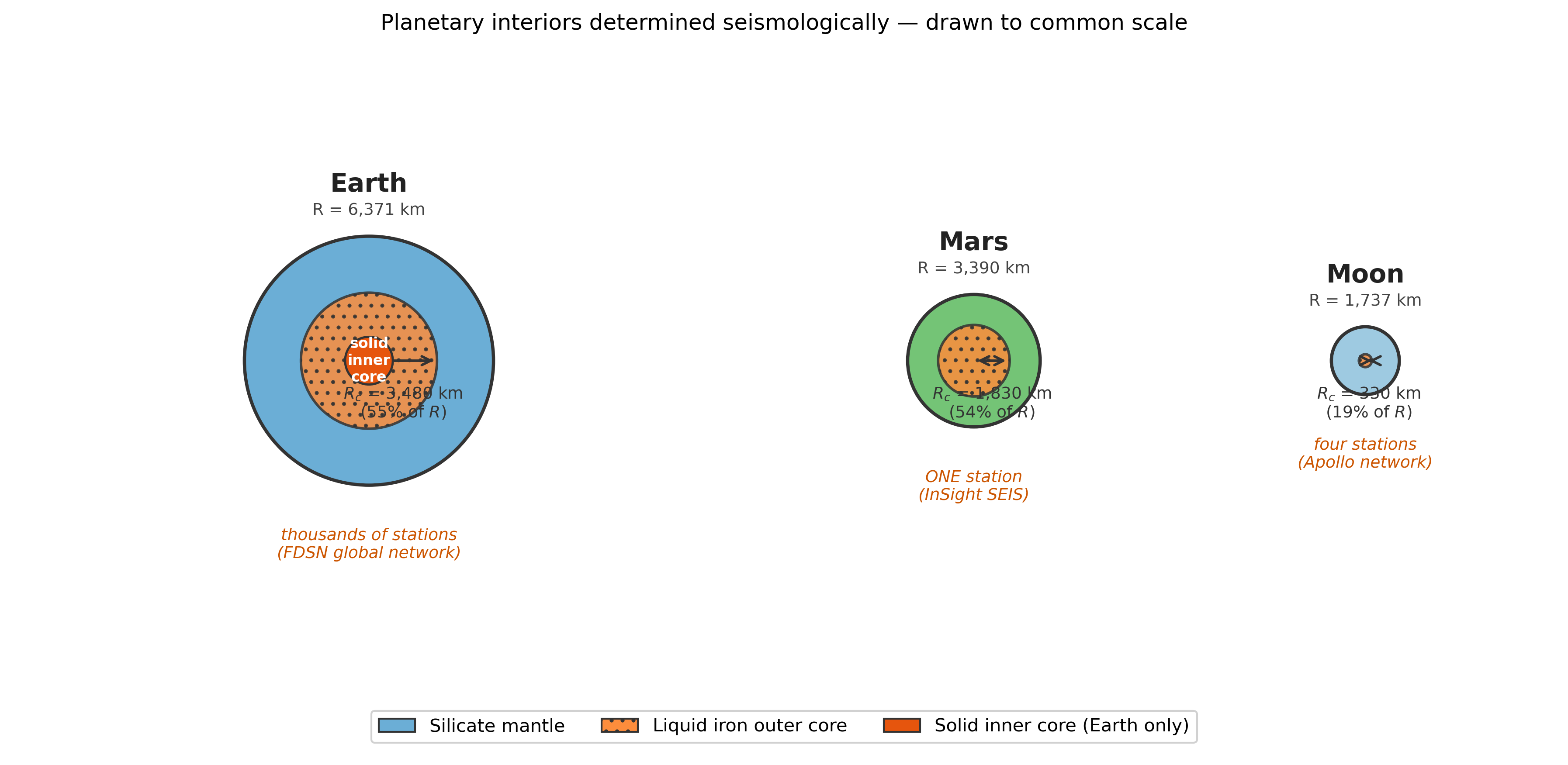— Fig. 163 The interiors of Earth, Mars, and the Moon to a common scale, each determined seismologically. Core size relative to planetary radius differs markedly, recording how much iron each body retained.#

8. AI Literacy: Evaluating a Synthesis Against Your Own Rubric#

AI Epistemics — the capstone standard (LO-7)

Throughout the course, AI assistance progressed from tutor, to writing coach, to something a scientist designs and supervises. The capstone test is the hardest: judging an AI-generated argument that spans several methods, where errors hide in the connections between facts rather than in the facts themselves.

A worked task. Prompt an AI assistant to “explain how geophysicists know the Earth’s outer core is liquid,” then evaluate the response against an explicit rubric before accepting any of it:

Mechanism stated correctly? The decisive evidence is the absence of direct S-waves through the core (the S-wave shadow), because a fluid has no shear strength. A response that cites only “the core is molten iron” without the seismological reasoning has stated a conclusion, not the evidence.
Independent observable acknowledged? A strong answer connects the seismological result to an independent constraint — the geodynamo requires a convecting electrical conductor, consistent with a liquid outer core. A response that treats one method as sufficient has missed the synthesis logic of this lecture.
Limits and uncertainty present? Does the response distinguish the liquid outer core from the solid inner core, and say how that distinction is made (PKIKP phases, normal modes)? Confident text that elides this is overclaiming.

The standard is not whether the AI sounds authoritative. It is whether its argument survives the same scrutiny applied to a research paper or a classmate’s reasoning. AI output is measured against the student’s own standard — not deferred to. Where the response fails a rubric item, that failure is recorded in the AI error log used in the AI Literacy lab.

Tip

Prompt Lab. Try the prompts below and grade each response against the three rubric items above before trusting it.

“Derive why oceanic seafloor deepens as the square root of its age.” (Check: does it invoke conductive cooling and isostasy, or assert the scaling without a mechanism?)
“Could gravity data alone determine the absolute thickness of the Martian crust?” (Check: does it identify the relative-versus-absolute degeneracy and the need for an independent seismic tie point?)
“Summarize the evidence that mantle plumes originate at the core–mantle boundary.” (Check: does it separate seismic imaging, geochemistry, and the deflection of plumes by mantle flow, or blend them into one unsupported claim?)

9. Concept Checks#

Gravity and seismic refraction are both proposed to map the depth to a basement interface beneath a sedimentary basin. State one property each method senses, and explain why running both is more informative than running either twice.
On the Moon, the core radius is about 19% of the planetary radius; on Mars it is about 54% (Fig. 163). Both figures were obtained seismologically. What does the contrast imply about how much iron each body retained relative to its silicate mantle?
The mantle’s Rayleigh number is of order \(10^{6}\text{–}10^{8}\), while the critical value is near \(10^{3}\). State, in one sentence each, what this implies about (a) how the mantle transfers heat and (b) why the conduction-only cooling model of section 3b is nonetheless valid in the lithosphere.
A volcanic island chain becomes progressively older away from an active volcano, yet lies far from any plate boundary. Explain why this observation cannot be accounted for by rigid-plate tectonics alone, and what the chain reveals about the mantle beneath. Why does a slowly migrating hotspot complicate using such chains as an absolute reference frame for plate motion?
The magnetic anomaly pattern reveals that a site on oceanic seafloor has age \(t = 40\) Ma. A heat-flow probe at the same site returns \(q = 45\ \mathrm{mW\,m^{-2}}\). (a) Compute the half-space predictions for heat flow and seafloor depth at 40 Ma (use \(q = 510\,t^{-1/2}\ \mathrm{mW\,m^{-2}}\) and \(d = 2500 + 350\,t^{1/2}\ \mathrm{m}\), with \(t\) in Ma). (b) The measured heat flow is roughly half the predicted value. Name one physical process that explains this discrepancy, and state why it is more prevalent over young seafloor than old. (c) The bathymetric depth at this site agrees well with the half-space prediction even though heat flow does not. Explain in one sentence why this joint result is more constraining than the heat-flow measurement alone.
A subduction-zone segment has seismically imaged dimensions \(L = 400\ \mathrm{km}\), \(W = 120\ \mathrm{km}\), and paleoseismic evidence indicates average coseismic slip \(\bar{D} = 8\ \mathrm{m}\). Using \(\mu = 30\ \mathrm{GPa}\): (a) compute \(M_0\) and \(M_w\); (b) identify two observing systems — from different methods — that together would determine whether rupture reached the seafloor in a future event; (c) explain in one sentence why that determination is critical for the tsunami prediction.

10. Connections#

Lecture 11 — Whole Earth I — seismic travel times and the reference velocity model that sections 3a–3b extend.
Lecture 12 — Seismic Tomography — the tomographic inverse problem of which (211) is a generalization.
Lecture 14 — Earthquake Phenomena I — the kinematics and dynamics of the seismic source, underpinning section 3d.
Lecture 16 — Focal Mechanisms — moment-tensor inversion as an instance of (211) with the elastic wave equation as forward operator.
Lecture 17 — Ground Motions — ground-motion prediction equations: the forward operator from \(M_0\) and site distance to engineering shaking intensity.
Lecture 18 — Tsunami — shallow-water wave propagation: the forward operator from fault slip to coastal run-up.
Lecture 19 — Earth’s Gravity — the Poisson equation forward operator in the \(\Delta g\) column of Fig. 161.
Lecture 21 — Isostasy — the isostatic balance that converts thermal contraction into seafloor deepening, (214).
Lecture 22 — Density of the Lithosphere — the density–temperature link connecting seismic velocity to gravity via the Nafe–Drake curve (section 3c).
Lecture 23 — Earth’s Magnetism — the magnetic forward operator and the Curie-point link between temperature and magnetization.
Lecture 25 — Magnetic Anomalies — seafloor spreading stripes as the source of age \(t\) entering (213) and (214).
Lecture 26 — Oceanic and Continental Lithosphere — the half-space cooling model derived and applied.
Lecture 28 — Convergent Margins — subduction as the cold downwelling limb of the convection engine; the seismic hazard synthesis of section 3d applied to Cascadia.

Putting It Together: Geophysics as a Tool for Earth Structure

Contents

Putting It Together: Geophysics as a Tool for Earth Structure#

Prerequisites#

1. The Geoscientific Question#

2. Governing Physics#

3. Mathematical Framework#

3a. The joint inverse problem#

3b. A concrete case: one thermal model, two observables#

3c. Seismic velocity and gravity: joint crustal imaging#

3d. Earthquake source, strong motion, and hazard: a multi-observable synthesis#

3e. From a cooling plate to a cooling planet#

4. Worked Example#

5. Connecting to Cascadia: From Local Cooling to the Global Engine#

Hotspots: where the rigid-plate picture breaks#

6. Scales of Investigation: Imaging the Subsurface from Planet to Pore#

6a. The scale ladder#

6b. The same logic at every depth#

6c. Why structure matters: resource management#

6d. Why structure matters: hazard modelling#

7. Research Horizon#

7a. Machine learning#

7b. Sensing technology#

7c. The cryosphere and the environment#

7d. Planetary interiors#

8. AI Literacy: Evaluating a Synthesis Against Your Own Rubric#

9. Concept Checks#

10. Connections#

Further Reading#