Seismic Wave Types

Seismic Wave Types#

1. The Geoscientific Question#

On January 26, 2014, a magnitude 4.3 earthquake struck near the town of Poulsbo, across Puget Sound from Seattle. Within seconds, seismometers at the Pacific Northwest Seismic Network (PNSN) recorded three distinct patterns of ground motion. The first arrival — a sharp, impulsive vertical jolt — came from a compressional wave that had traveled directly through the crust. Several seconds later, a stronger horizontal shake arrived: a shear wave, moving more slowly but carrying more destructive energy. Finally, a long, rolling oscillation built up and persisted for over a minute — surface waves, trapped near the Earth’s free surface and spreading outward like ripples on a pond.

These three wave types are not separate phenomena. They are different solutions to the same elastic wave equation derived in Lecture 3. The equation of motion, \(\rho\,\partial^2\mathbf{u}/\partial t^2 = (\lambda+2\mu)\nabla(\nabla\cdot\mathbf{u}) - \mu\nabla\times(\nabla\times\mathbf{u})\), contains within it the seeds of all seismic wave behavior: the P-wave, the S-wave, and — when boundary conditions at the free surface are imposed — the Rayleigh and Love surface waves.

This lecture classifies the four seismic wave types, explains their particle motions and speed relationships, and introduces the \(V_P/V_S\) ratio as one of the most powerful diagnostic tools in applied geophysics. The question driving the lecture is: Given a single earthquake source, why does the Earth produce such different kinds of shaking, and what does each one reveal about the subsurface?

The Central Question

The elastic wave equation admits multiple solution families with distinct particle motions and speeds. Each wave type carries different information about the subsurface. How do seismologists use these differences to probe Earth structure?

2. Governing Physics: From the Wave Equation to Wave Types#

2.1 The Helmholtz Decomposition#

The vector equation of motion derived in Lecture 3 governs the displacement field \(\mathbf{u}(\mathbf{x}, t)\) in a homogeneous, isotropic, elastic solid:

(27)#\[ \rho\,\frac{\partial^2\mathbf{u}}{\partial t^2} = (\lambda+2\mu)\,\nabla(\nabla\cdot\mathbf{u}) - \mu\,\nabla\times(\nabla\times\mathbf{u}) \]

The Helmholtz theorem states that any sufficiently smooth vector field can be decomposed into an irrotational (curl-free) part and a solenoidal (divergence-free) part:

(28)#\[ \mathbf{u} = \nabla\phi + \nabla\times\boldsymbol{\psi} \]

where \(\phi(\mathbf{x},t)\) is a scalar potential and \(\boldsymbol{\psi}(\mathbf{x},t)\) is a vector potential with \(\nabla\cdot\boldsymbol{\psi} = 0\). Substituting (28) into (27) and using the vector identity \(\nabla\times(\nabla\phi) = 0\) and \(\nabla\cdot(\nabla\times\boldsymbol{\psi}) = 0\) separates the equation into two independent wave equations:

(29)#\[ \frac{\partial^2\phi}{\partial t^2} = V_P^2\,\nabla^2\phi, \qquad V_P = \sqrt{\frac{\lambda+2\mu}{\rho}} \]

(30)#\[ \frac{\partial^2\boldsymbol{\psi}}{\partial t^2} = V_S^2\,\nabla^2\boldsymbol{\psi}, \qquad V_S = \sqrt{\frac{\mu}{\rho}} \]

Key Concept: Two Independent Wave Families

The Helmholtz decomposition splits the elastic wavefield into two non-interacting wave families in a homogeneous medium:

Dilatational waves (P-waves): governed by \(\phi\), involving volume change (\(\nabla\cdot\mathbf{u} \neq 0\)), no rotation (\(\nabla\times\mathbf{u} = 0\)).
Rotational waves (S-waves): governed by \(\boldsymbol{\psi}\), involving shape change only (\(\nabla\cdot\mathbf{u} = 0\)), no volume change.

These two families propagate independently at different speeds. They couple only at boundaries between media with different properties — a fact that will become central in Lectures 6 and 7.

2.2 Why Two Wave Speeds?#

The physical reason for two distinct wave types traces back to the two independent modes of elastic deformation introduced in Lecture 3: volumetric strain (resisted by \(K\) and \(\lambda\)) and shear strain (resisted by \(\mu\)). A P-wave compresses and dilates the medium along its propagation direction, engaging both bulk and shear resistance — hence the P-wave modulus is \(M = \lambda + 2\mu = K + \frac{4}{3}\mu\). An S-wave distorts the medium without changing its volume, engaging only the shear modulus \(\mu\). Since \(\lambda + 2\mu > \mu\) for any stable elastic material, P-waves are always faster than S-waves.

3. Mathematical Framework#

3.1 Notation#

Notation

Symbol	Quantity	Units	Type
\(\mathbf{u}\)	Displacement vector	m	vector
\(\phi\)	Scalar displacement potential (P-wave)	m²	scalar
\(\boldsymbol{\psi}\)	Vector displacement potential (S-wave)	m²	vector
\(V_P\)	P-wave velocity	m/s	scalar
\(V_S\)	S-wave velocity	m/s	scalar
\(V_R\)	Rayleigh wave phase velocity	m/s	scalar
\(\Gamma\)	\(V_P/V_S\) ratio	dimensionless	scalar
\(\nu\)	Poisson’s ratio	dimensionless	scalar
\(\lambda\)	First Lamé parameter	Pa	scalar
\(\mu\)	Shear modulus	Pa	scalar
\(\rho\)	Density	kg/m³	scalar
\(k\)	Wavenumber \(= 2\pi/\lambda_\text{dom}\)	m⁻¹	scalar
\(\lambda_\text{dom}\)	Dominant wavelength	m	scalar
\(f\)	Frequency	Hz	scalar
\(T\)	Period	s	scalar
\(Z\)	Acoustic impedance \(= \rho V\)	kg/(m²·s) = Pa·s/m	scalar

3.2 Body Waves#

P-waves (Primary, Compressional, Longitudinal). Particle motion is parallel to the propagation direction. The medium alternately compresses (particles crowd together) and rarefies (particles spread apart), creating a traveling pattern of density fluctuations — conceptually similar to sound waves in air. P-waves propagate through any material that resists compression: solids, liquids, and gases.

(31)#\[ V_P = \sqrt{\frac{\lambda + 2\mu}{\rho}} = \sqrt{\frac{K + \frac{4}{3}\mu}{\rho}} \]

S-waves (Secondary, Shear, Transverse). Particle motion is perpendicular to the propagation direction. No volume change occurs — the medium distorts in shape without compression or dilation. S-waves require a material with nonzero shear modulus: they propagate through solids but not through fluids.

(32)#\[ V_S = \sqrt{\frac{\mu}{\rho}} \]

P-wave particle motion diagram. Particles are shown as colored dots along a horizontal line. Clusters of close-spaced blue dots represent compression zones labeled C; clusters of wide-spaced sky-blue dots represent rarefaction zones labeled R. Orange horizontal arrows above the particle row show that displacement is parallel to the propagation direction (left to right), which is indicated by a labeled arrow at the top right. 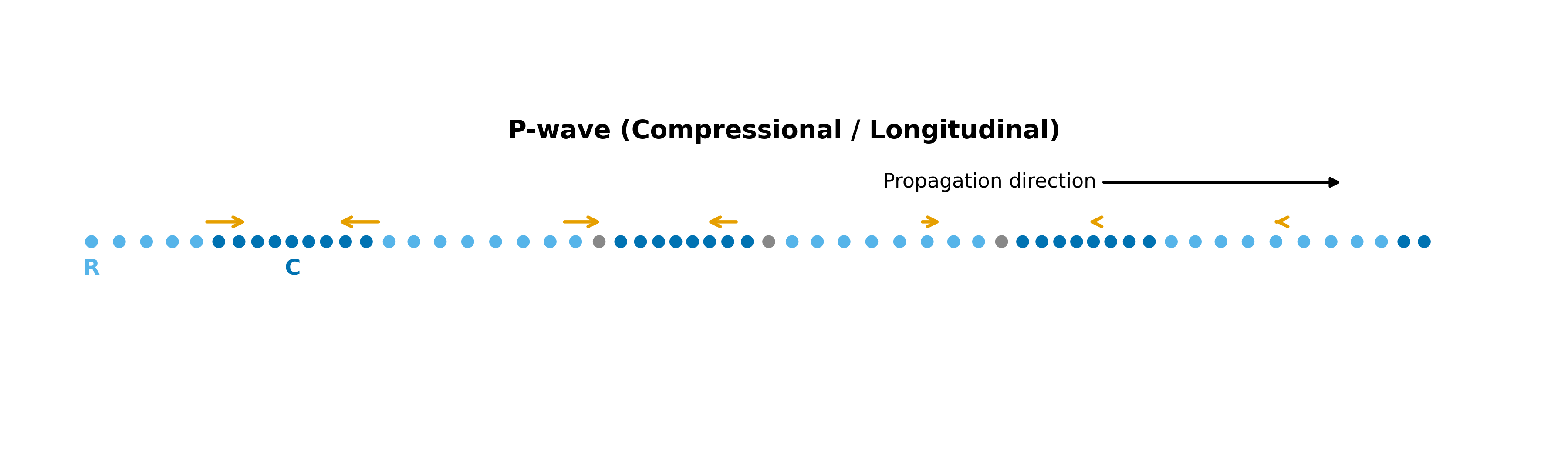— Fig. 9 **Figure 4.1.** P-wave (compressional / longitudinal) particle motion. Compression zones (C, blue) and rarefaction zones (R, sky blue) alternate along the propagation direction; particle displacement (orange arrows) is parallel to propagation. [Python-generated. Script: `assets/scripts/fig_pwave_swave_motion.py`]#

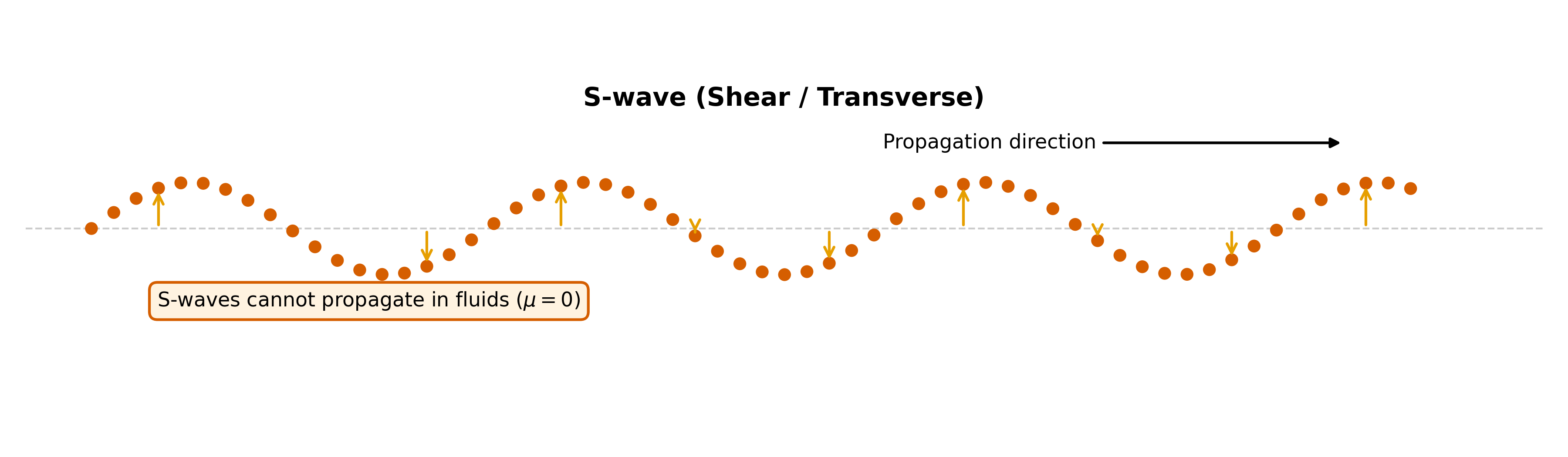
S-wave particle motion diagram. Vermilion particles trace a sinusoidal path above and below a dashed horizontal equilibrium line. Orange vertical arrows show that particle displacement is perpendicular to the propagation direction (left to right, indicated by a labeled arrow at top right). A callout box notes that S-waves cannot propagate in fluids because the shear modulus mu equals zero. — Fig. 10 **Figure 4.2.** S-wave (shear / transverse) particle motion. Particles oscillate perpendicular to the propagation direction (orange arrows), with no volume change. S-waves require a nonzero shear modulus and therefore do not propagate in fluids. [Python-generated. Script: `assets/scripts/fig_pwave_swave_motion.py`]#

3.3 S-Wave Polarization: SV and SH#

The S-wave displacement is confined to the plane perpendicular to the ray direction — a plane that has two independent directions. Seismologists decompose the S-wave into two polarization components:

SV (Shear-Vertical): Particle motion lies in the vertical plane containing the ray. SV waves interact with the free surface and with horizontal interfaces to generate Rayleigh waves and to undergo mode conversion to P-waves.

SH (Shear-Horizontal): Particle motion is horizontal, perpendicular to both the ray and the vertical plane. SH waves do not convert to P-waves at horizontal interfaces. Constructive interference of SH waves trapped in a low-velocity surface layer produces Love waves.

Three-dimensional diagram showing a ray propagating downward and to the right. The propagation direction is labeled P with a blue arrow. A vertical plane containing the ray is shaded light blue. The SV polarization is shown as a vermilion double-headed arrow within this vertical plane, perpendicular to the ray. The SH polarization is shown as an amber double-headed arrow perpendicular to both the ray and SV, pointing horizontally out of the vertical plane. The three directions P, SV, SH form an orthogonal triad. 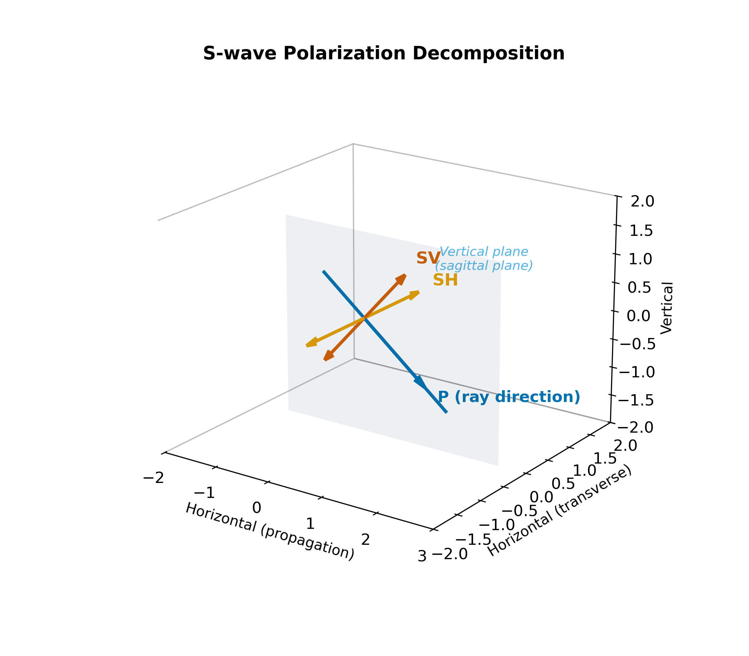— Fig. 11 **Figure 4.3.** Decomposition of S-wave polarization into SV (in the vertical plane containing the ray) and SH (horizontal, out of the ray plane). Together with the P-wave direction, these define an orthogonal coordinate system aligned with the ray. [Python-generated. Script: `assets/scripts/fig_sv_sh_polarization.py`]#

The SV–SH decomposition is not merely a mathematical convenience. It reflects a physical asymmetry: the free surface and horizontal layering break the symmetry between vertical and horizontal transverse motions. An SV wave arriving at the surface generates both vertical and horizontal ground motion; an SH wave generates only horizontal motion. This distinction directly determines which surface wave types are excited.

3.4 The \(V_P/V_S\) Ratio and Poisson’s Ratio#

The ratio of P-wave to S-wave speed is one of the most diagnostic quantities in geophysics:

(33)#\[ \Gamma = \frac{V_P}{V_S} = \sqrt{\frac{\lambda + 2\mu}{\mu}} \]

This ratio depends only on the Lamé parameters (or equivalently, on Poisson’s ratio), not on density. The connection to Poisson’s ratio \(\nu\) is:

(34)#\[ \Gamma = \sqrt{\frac{2(1-\nu)}{1-2\nu}} \]

and inversely:

(35)#\[ \nu = \frac{\Gamma^2 - 2}{2(\Gamma^2 - 1)} \]

Key Equation: \(V_P/V_S\) and Poisson’s Ratio

\[ \frac{V_P}{V_S} = \sqrt{\frac{2(1-\nu)}{1-2\nu}} \]

Physical limits:

\(\nu = 0.25\) (a Poisson solid): \(V_P/V_S = \sqrt{3} \approx 1.73\) — a common approximation for crustal rock.
\(\nu \to 0.5\) (incompressible fluid): \(V_P/V_S \to \infty\) — the S-wave speed vanishes.
\(\nu = 0\) (no lateral expansion under compression): \(V_P/V_S = \sqrt{2} \approx 1.41\) — the minimum possible ratio for a stable elastic solid.

Anomalously high \(V_P/V_S\) (> 2.0) indicates fluid saturation, partial melt, or very high pore pressure. This is the basis for detecting fluids in sedimentary basins, magma chambers, and fault zones.

Units check: \([V_P/V_S] = (\text{m/s})/(\text{m/s}) = \text{dimensionless}\) ✓. Poisson’s ratio is also dimensionless ✓.

3.5 Seismic Velocities of Earth Materials#

Seismic wave speeds span nearly two orders of magnitude across common Earth materials:

Horizontal bar chart. Vertical axis lists Earth materials grouped by category: crystalline rocks (granite at 5200, basalt at 5900, limestone at 4000 to 7000, sandstone at 2000 to 5500, salt rock at 4600 meters per second), unconsolidated sediments (dry sand at 120 to 270, wet sand at 200 to 800, clay V_S at 60 to 150 meters per second), fluids (seawater at 1530, freshwater at 1480 meters per second), and engineering materials (steel at 5900, aluminum at 6400, ice at 3000 to 4000 meters per second). Horizontal axis shows V_P in meters per second from 0 to 8000. Bars are colored by category using the colorblind-safe palette. 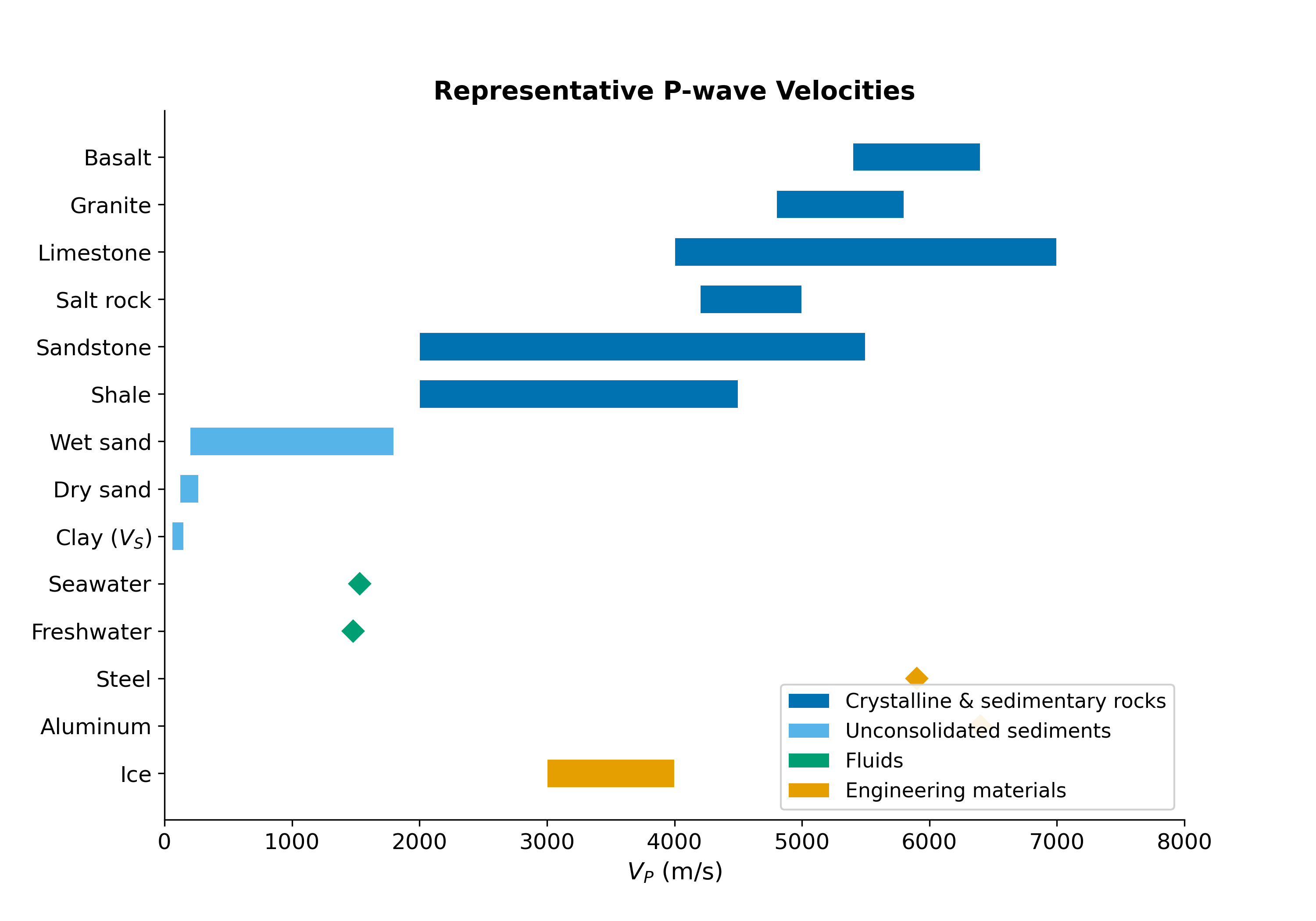— Fig. 12 **Figure 4.3.** Representative P-wave velocities for Earth and engineering materials. The enormous range from ~60 m/s (soft clay shear velocity) to ~6500 m/s (basalt) reflects the wide variation in elastic moduli and density across geological materials. [Python-generated. Script: `assets/scripts/fig_seismic_velocities.py`]#

The controls on velocity are straightforward from the expressions \(V_P = \sqrt{(\lambda+2\mu)/\rho}\) and \(V_S = \sqrt{\mu/\rho}\):

Stiffness increases velocity. Crystalline rocks (high \(\mu\), high \(K\)) are fast. Unconsolidated sediments (low \(\mu\), low \(K\)) are slow. Cementation, compaction, and mineral composition all increase stiffness and therefore velocity.

Density increases velocity indirectly. Higher density alone would decrease velocity (it appears in the denominator). But in practice, denser rocks are also stiffer, and the stiffness increase dominates. The net effect is that velocity generally increases with density across rock types — a relationship known as Birch’s law.

Fluid saturation affects P and S differently. Filling pores with water increases \(K\) (water is much less compressible than air) but does not increase \(\mu\) (water has zero shear modulus). The result: \(V_P\) increases upon saturation, while \(V_S\) is nearly unchanged or decreases slightly. This asymmetric response is why the \(V_P/V_S\) ratio is such a powerful fluid indicator.

Pressure increases velocity; temperature decreases it. With depth in the Earth, confining pressure closes microcracks and stiffens grain contacts, increasing velocity. Temperature weakens grain contacts and approaches partial melt conditions, decreasing velocity. The competition between these effects creates the complex velocity-depth profiles observed in the real Earth.

3.6 Surface Waves#

Surface waves arise when body waves interact with the Earth’s free surface. The boundary condition — zero traction at the surface (\(\sigma_{iz} = 0\) at \(z = 0\)) — admits solutions whose amplitude decays exponentially with depth, concentrating energy near the surface.

Rayleigh Waves. Rayleigh waves combine P and SV motion to satisfy the free-surface boundary condition. Particles at the surface trace retrograde elliptical orbits — they move backward (opposite to the propagation direction) at the wave crest and forward in the trough. The ellipse axes shrink with depth, and the motion reverses to prograde below a depth of approximately \(0.2\lambda_\text{dom}\), becoming negligible by \(\sim 0.4\lambda_\text{dom}\).

The Rayleigh wave speed in a homogeneous half-space is:

(36)#\[ V_R \approx \frac{0.87 + 1.12\nu}{1 + \nu}\,V_S \]

For a Poisson solid (\(\nu = 0.25\)): \(V_R \approx 0.92\,V_S\).

Love Waves. Love waves are purely horizontal (SH polarization). They require a velocity gradient — specifically, a slower surface layer over a faster half-space with \(V_{S1} < V_{S2}\). SH waves incident on the base of the slow layer at angles beyond the critical angle undergo total internal reflection and become trapped, bouncing between the free surface and the base of the layer. Constructive interference of these trapped reflections produces the Love wave. The Love wave phase velocity is bounded:

(37)#\[ V_{S1} < V_\text{Love} < V_{S2} \]

Three-panel figure. Left panel shows Rayleigh wave particle motion at five depths, with retrograde ellipses at the surface that shrink and reverse to prograde at depth, and a vertical dashed line marking the surface. Center panel shows Rayleigh wave amplitude versus depth as an exponentially decaying curve, with a horizontal dashed line at 0.4 wavelength depth labeled as the approximate depth of significance, and the phase velocity labeled as V_R approximately 0.92 V_S. Right panel shows a cross-section with a light blue slow surface layer of thickness H over a green fast half-space, with orange zigzag arrows representing SH wave paths bouncing between the free surface and the layer base by total internal reflection, and horizontal dots representing transverse particle motion perpendicular to the propagation direction. 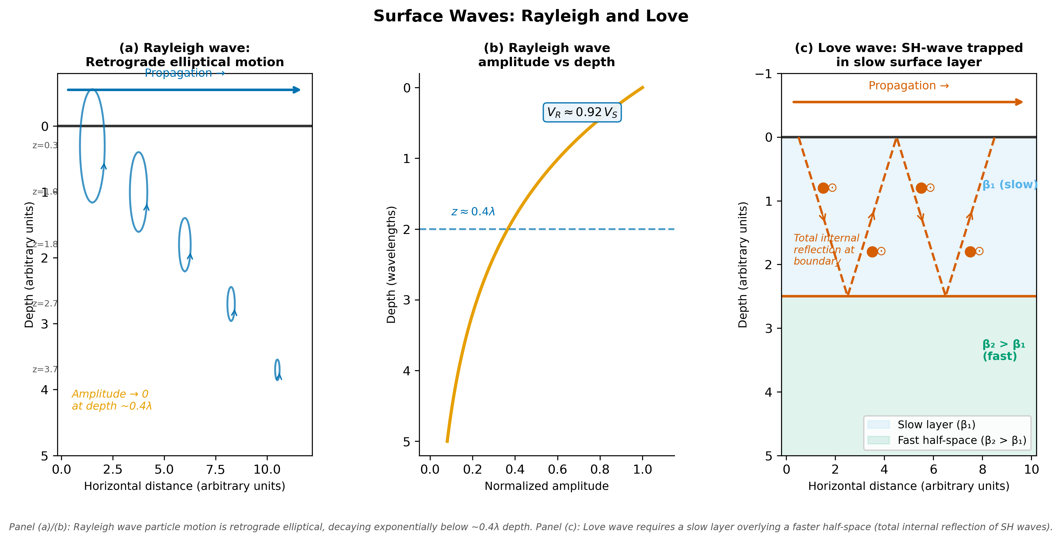— Fig. 13 **Figure 4.4.** Surface waves. Left and center: Rayleigh wave retrograde elliptical motion and amplitude decay with depth. Right: Love wave formation by SH trapping in a slow surface layer via total internal reflection at the base. [Python-generated. Script: `assets/scripts/fig_surface_waves.py`]#

Key Concept: Surface Wave Dispersion

Both Rayleigh and Love waves are dispersive in a layered Earth: their phase velocity depends on frequency. Longer-period waves penetrate deeper and sample faster material, so they travel faster. Shorter-period waves are confined to the shallow, slow layer and travel more slowly. Measuring how phase velocity changes with period — the dispersion curve — is the basis for surface wave tomography, one of the most powerful tools for imaging the crust and upper mantle. The physics is straightforward: each period samples a different depth range of \(V_S(z)\), so the dispersion curve is effectively a depth-averaged \(V_S\) profile.

3.7 Wave Type Summary#

Wave Type Summary Table

Wave type	Particle motion	Speed	Propagates in fluids?	Key diagnostic
P (Primary)	Parallel to propagation (longitudinal)	\(V_P = \sqrt{(\lambda+2\mu)/\rho}\)	Yes	Fastest arrival; sensitive to both \(K\) and \(\mu\)
S (Secondary)	Perpendicular to propagation (transverse)	\(V_S = \sqrt{\mu/\rho}\)	No (\(\mu = 0\) in fluids)	Sensitive to shear rigidity only; key for site characterization
Rayleigh	Retrograde elliptical (P + SV), in vertical plane	\(V_R \approx 0.92\,V_S\)	Surface of solid only	Dispersive; dominant ground motion at distance
Love	Horizontal transverse (SH)	\(V_{S1} < V_\text{Love} < V_{S2}\)	Requires slow-over-fast layering	Dispersive; pure horizontal shaking

4. The Forward Problem#

Given the elastic properties of a subsurface model — \(\lambda(\mathbf{x})\), \(\mu(\mathbf{x})\), \(\rho(\mathbf{x})\) — the forward problem predicts:

Model parameters: \(\lambda\), \(\mu\), \(\rho\) as functions of position (or equivalently \(V_P\), \(V_S\), \(\rho\))

Observables predicted:

Wave speeds \(V_P(\mathbf{x}) = \sqrt{(\lambda+2\mu)/\rho}\) and \(V_S(\mathbf{x}) = \sqrt{\mu/\rho}\) at each point
The arrival order and timing of P, S, and surface waves at a seismometer
The particle motion (polarization) recorded on each component of a three-component seismometer
Surface wave dispersion curves \(c(T)\) from the depth-dependent velocity structure

See companion notebook: notebooks/Lab1-Intro-Python.ipynb — students compute \(V_P\) and \(V_S\) for various rock types from tabulated moduli and density.

5. The Inverse Problem#

Inverse Problem Setup

Data \(d\): Observed arrival times of P, S, and surface waves; surface wave dispersion curves; particle motion polarizations
Model \(m\): \(V_P(\mathbf{x})\), \(V_S(\mathbf{x})\), \(\rho(\mathbf{x})\)
Forward relation: \(d = G(m)\) maps the velocity model to predicted travel times and waveforms via the wave equation
Key non-uniqueness: Travel times constrain only \(V_P\) and \(V_S\), not \(\lambda\), \(\mu\), and \(\rho\) separately. To distinguish between a density increase and a modulus increase, additional data (amplitudes, gravity) are needed.
Resolution limits: Only structures larger than the dominant wavelength \(\lambda_\text{dom} = V/f\) are resolvable. At 1 Hz and \(V_P = 6\) km/s, the wavelength is 6 km — structures smaller than this are invisible to teleseismic body waves.

6. Worked Examples#

6.1 The S–P Time Method for Earthquake Distance#

A seismogram at PNSN station SEW (Seattle, near the UW campus) records the Poulsbo M4.3 earthquake with P-wave arrival at 04:12:07.2 UTC and S-wave arrival at 04:12:11.8 UTC.

\[ \Delta t_{S-P} = t_S - t_P = 11.8 - 7.2 = 4.6 \text{ s} \]

Assuming average crustal velocities \(V_P = 6.3\) km/s and \(V_P/V_S = 1.73\):

\[ V_S = \frac{6.3}{1.73} = 3.64 \text{ km/s} \]

Distance from the formula \(d = \Delta t \cdot \frac{V_P V_S}{V_P - V_S}\):

\[ d = 4.6 \times \frac{6.3 \times 3.64}{6.3 - 3.64} = 4.6 \times \frac{22.93}{2.66} = 4.6 \times 8.62 \approx 39.7 \text{ km} \]

This is consistent with the straight-line distance from Poulsbo to the UW campus (~40 km). The method works because P- and S-waves travel at different speeds through the same rock — the time difference grows linearly with distance.

6.2 \(V_P/V_S\) as a Fluid Diagnostic#

A shallow borehole in the Duwamish Valley (south Seattle) logs \(V_P = 1750\) m/s and \(V_S = 220\) m/s in a layer of Holocene alluvium at 15 m depth.

\[ \Gamma = \frac{V_P}{V_S} = \frac{1750}{220} = 7.95 \]

\[ \nu = \frac{\Gamma^2 - 2}{2(\Gamma^2 - 1)} = \frac{63.2 - 2}{2(63.2 - 1)} = \frac{61.2}{124.4} = 0.492 \]

This Poisson’s ratio is extremely close to the incompressible limit of 0.5. The interpretation: these alluvial sediments are fully water-saturated, with the P-wave speed dominated by the pore fluid (\(V_P \approx 1500\) m/s for water) and the S-wave speed controlled by the extremely weak grain-to-grain contacts in unconsolidated sediment. This condition is directly responsible for the severe ground-motion amplification observed in this part of Seattle during the 2001 Nisqually earthquake.

Concept Check

A basalt sample has \(V_P = 5900\) m/s and \(V_S = 3200\) m/s. Calculate \(V_P/V_S\) and Poisson’s ratio. Is this consistent with a dry, crystalline rock?
Explain in two sentences — without using the formula — why S-waves cannot propagate through water. The explanation should reference a specific physical process at the molecular scale.
A Love wave at period \(T = 5\) s has phase velocity 2.8 km/s, and at \(T = 20\) s has phase velocity 3.6 km/s. (a) What does this dispersion tell us about how \(V_S\) changes with depth? (b) Estimate the depth sampled by each period using the approximation depth \(\approx 0.4\,V_R\,T\).
An AI assistant claims that “P-waves are faster than S-waves because they involve compression, which is faster than shearing.” Critique this statement. Is “compression is faster” a physical explanation? What does the speed ratio \(\sqrt{(\lambda+2\mu)/\mu}\) actually tell us about why P-waves are faster?

7. Course Connections#

Prior lecture (Lecture 3): The wave equation derived in Lecture 3 is the starting point for everything in this lecture. The elastic moduli and their physical interpretation appear here as the controls on wave speed and wave type.
Lecture 6 (Wavefronts, Rays, and Snell’s Law): The wave speeds \(V_P\) and \(V_S\) derived here become the velocities \(V_1\) and \(V_2\) in Snell’s law. The concept of distinct P- and S-wave speeds is essential for understanding mode conversion at boundaries.
Lecture 7 (Waves at Boundaries): The SV/SH decomposition introduced here determines which modes convert at interfaces. The \(V_P/V_S\) ratio controls the reflection coefficient and impedance contrast.
Lectures 9–11 (Seismic Refraction): The velocity table (§3.5) provides the geological context for choosing velocity models in refraction interpretation.
Lectures 17–18 (Whole Earth Structure): The S-wave shadow zone — S-waves are absent at epicentral distances > 104° — is the primary evidence that the outer core is liquid (\(\mu = 0\)). The physics is directly from §3.2.
Lab 1 (Apr 3): Students compute \(V_P\), \(V_S\), and \(V_P/V_S\) from tabulated elastic moduli and density for a suite of rock types, plot the results, and interpret geological trends.
Cross-topic link: Surface wave dispersion (§3.6) reappears in the gravity module: surface waves sensitive to \(V_S(z)\) provide density-independent constraints on crustal structure that complement gravity observations, which sense \(\rho(z)\) directly.

8. Research Horizon#

Current Research Highlights (2022–2025)

Distributed Acoustic Sensing (DAS) and urban surface wave tomography. DAS converts fiber-optic telecommunication cables into dense seismic arrays with channel spacing of a few meters over tens of kilometers. Cheng et al. (2023, JGR: Solid Earth, doi:10.1029/2023JB026957) used dark fiber in the Imperial Valley (California) to perform ambient-noise surface wave tomography at basin scale, retrieving \(V_S\) structure down to several hundred meters with lateral resolution of ~100 m. The physics is the same dispersion analysis described in §3.6 — each frequency samples a different depth through the Rayleigh wave sensitivity kernel — but the data density from DAS is orders of magnitude beyond conventional seismometer networks. Emily Wilbur, the TA for this course, uses DAS in her own research on shallow structure in the Pacific Northwest.

Machine-learning seismic phase identification. Deep-learning models such as PhaseNet and EQTransformer now achieve near-human accuracy in automatically identifying P- and S-wave arrivals on continuous seismic records. These models exploit the same physical differences described in §3.2: P-waves produce primarily vertical motion with higher-frequency content, while S-waves produce stronger horizontal motion at lower frequencies. Münchmeyer et al. (2022, Journal of Geophysical Research: Solid Earth, doi:10.1029/2021JB023499) benchmarked seven such models on a common dataset and found that transformer-based architectures achieve the best generalization across different tectonic settings. The relevance for this course: the physics that distinguishes wave types is the same physics embedded (implicitly) in the training data of these models.

Vp/Vs monitoring for volcanic unrest. Temporal changes in \(V_P/V_S\) beneath active volcanoes serve as precursors to eruption. An increase in \(V_P/V_S\) can indicate rising pore fluid pressure or the arrival of new melt into a magma reservoir — both increase \(V_P/V_S\) by the mechanisms described in §3.4. Brenguier et al. (2023, Nature Reviews Earth & Environment, doi:10.1038/s43017-022-00374-y (⚠ DOI returns 404 — verify manually)) reviewed how ambient noise monitoring recovers temporal velocity changes at sub-percent precision, enabling detection of pre-eruptive inflation. The same \(\mu = 0\) physics that prevents S-waves from entering the outer core also produces anomalously high \(V_P/V_S\) in partially molten zones beneath volcanoes.

For students interested in this area: The IRIS SSBW (Seismology Skill Building Workshop) covers hands-on phase picking and surface wave analysis with ObsPy each summer. See iris.edu/hq/workshops.

9. Societal Relevance#

Why It Matters: ShakeAlert and Ground Motion Amplification

ShakeAlert: using P-waves to save lives. The USGS ShakeAlert earthquake early warning system detects P-wave arrivals at near-source seismometers and issues alerts before the more damaging S-waves and surface waves arrive at distant population centers. For a Cascadia M9 earthquake, the P-wave reaches the coast of Washington ~15 seconds after rupture begins; the strong S-wave shaking reaches Seattle 60–90 seconds later. That interval — determined entirely by the \(V_P > V_S\) relationship from §3.2 — is the warning window. It is enough time to stop trains, open fire station doors, pause surgeries, and move away from windows. ShakeAlert became fully operational in Washington State in May 2021 and has issued several public alerts for Pacific Northwest earthquakes since then.

\(V_{S30}\) and building codes. The average shear-wave velocity in the top 30 meters of soil — denoted \(V_{S30}\) — is the primary parameter used in the International Building Code (IBC/ASCE 7) to classify seismic site conditions. The classification ranges from Site Class A (\(V_{S30} > 1500\) m/s, hard rock) to Site Class E (\(V_{S30} < 180\) m/s, soft soil). The design earthquake force for a building on Site Class E soil can be three to five times larger than on Site Class B rock, because the impedance contrast amplifies ground motion by the physics of §3.4. In Seattle, the difference between a Capitol Hill site (glacial till, \(V_{S30} \approx 500\) m/s) and a Pioneer Square site (Holocene fill, \(V_{S30} \approx 180\) m/s) determines whether a building is designed for moderate or severe shaking.

For further exploration:

ShakeAlert system status and Pacific Northwest coverage: shakealert.org
USGS site amplification factors and \(V_{S30}\) maps: earthquake.usgs.gov/hazards/vs30
PNSN real-time earthquake monitoring: pnsn.org

AI Literacy#

AI as a Tool: Machine Learning for Seismic Phase Picking

Identifying P-wave and S-wave arrivals on seismograms — phase picking — is one of the oldest tasks in seismology and one of the first to be substantially automated by deep learning. Models like PhaseNet (Zhu & Beroza, 2019) and EQTransformer (Mousavi et al., 2020) process continuous waveform data and output probability functions for P and S arrival times.

These models succeed because they exploit the same physics from this lecture: P arrivals are impulsive, often dominant on the vertical component, and have higher-frequency content. S arrivals are emergent, dominant on horizontal components, and richer in low-frequency energy. The neural network learns these patterns from millions of labeled picks — but the patterns are the wave physics.

Limitations to evaluate critically: ML pickers can fail on unusual waveforms: deep events with long-period P arrivals, mine blasts with different source radiation, or stations with unusual site effects. The model has no physical understanding — it has learned statistical correlations. When a waveform falls outside the training distribution, the model can produce confident but wrong picks.

LO-7 connection: When using an AI tool for phase picking (or any automated seismological analysis), the question is always: “Does the output make physical sense?” The \(V_P/V_S\) ratio provides a direct check: if the picked S–P time implies a \(V_P/V_S\) ratio outside the physically plausible range (roughly 1.4–2.5 for crustal rock), something is wrong with the pick.

AI Prompt Lab

Prompt 1 — Physical explanation:

“Explain why S-waves cannot propagate through liquid water. Do not just cite the formula V_S = sqrt(mu/rho) with mu = 0. Instead, explain at the molecular level what happens when a transverse disturbance is applied to a liquid, and why no restoring force develops.”

Evaluate: Does the AI correctly distinguish between elastic restoring forces (which require a structured lattice that resists shear) and viscous resistance (which dissipates energy rather than storing it)? A common error is to conflate “fluids resist shear” (they do, viscously, at finite strain rates) with “fluids have zero shear modulus” (true only in the elastic, zero-frequency limit).

Prompt 2 — Quantitative check:

“A sediment has lambda = 2.5 GPa, mu = 0.15 GPa, and density = 1900 kg/m³. Calculate V_P, V_S, V_P/V_S, and Poisson’s ratio. Interpret the results in terms of fluid saturation and sediment consolidation.”

Evaluate: Does the AI get \(V_P = \sqrt{(2.5 + 0.3) \times 10^9 / 1900} \approx 1220\) m/s? Does it get \(V_S = \sqrt{0.15 \times 10^9/1900} \approx 281\) m/s? \(V_P/V_S \approx 4.3\)? Does it correctly identify this as a partially saturated or very soft sediment based on the high \(V_P/V_S\)?

Prompt 3 — Failure mode test:

“Is it true that Rayleigh waves are always slower than S-waves?”

Evaluate: In a homogeneous half-space, yes (\(V_R \approx 0.92\,V_S\)). But in a layered medium, the Rayleigh wave phase velocity is dispersive and can vary. Does the AI note this subtlety, or does it give a blanket answer? A well-calibrated response would say “yes, in a homogeneous half-space” and note that layering introduces dispersion.

References#

@book{lowrie2020,
  author    = {Lowrie, W. and Fichtner, A.},
  title     = {Fundamentals of Geophysics},
  edition   = {3rd},
  publisher = {Cambridge University Press},
  year      = {2020},
  doi       = {10.1017/9781108685917}
}

@misc{mitocw12201,
  author = {Van Der Hilst, R.},
  title  = {12.201 Essentials of Geophysics, \S4.6--4.8},
  year   = {2004},
  note   = {MIT OpenCourseWare, CC BY NC SA},
  url    = {https://ocw.mit.edu/courses/12-201-essentials-of-geophysics-fall-2004}
}

@misc{iris_animations,
  title  = {{IRIS EarthScope Seismic Wave Animations}},
  note   = {CC BY 4.0},
  url    = {https://www.iris.edu/hq/inclass/animation/seismic_wave_motions4_waves_animated}
}

@misc{braile2009,
  author = {Braile, L. W.},
  title  = {Seismic Waves and the Slinky},
  year   = {2009},
  note   = {IRIS Educational Resource, CC BY},
  url    = {https://www.iris.edu/hq/cd_fall_2009/files/materials/Educational\%20Resources/slinky4.pdf}
}

@article{cheng2023,
  author  = {Cheng, F. and Ajo-Franklin, J. B. and others},
  title   = {High-Resolution Near-Surface Imaging at the Basin Scale Using Dark Fiber and Distributed Acoustic Sensing},
  journal = {Journal of Geophysical Research: Solid Earth},
  volume  = {128},
  number  = {9},
  year    = {2023},
  doi     = {10.1029/2023JB026957}
}

@article{munchmeyer2022,
  author  = {M{\"u}nchmeyer, J. and others},
  title   = {Which Picker Fits My Data? A Quantitative Evaluation of Deep Learning Based Seismic Pickers},
  journal = {Journal of Geophysical Research: Solid Earth},
  volume  = {127},
  number  = {1},
  year    = {2022},
  doi     = {10.1029/2021JB023499}
}

@article{brenguier2023,
  author  = {Brenguier, F. and others},
  title   = {Noise-based monitoring of volcanoes and faults},
  journal = {Nature Reviews Earth \& Environment},
  volume  = {4},
  pages   = {312--326},
  year    = {2023},
  doi     = {10.1038/s43017-022-00374-y} % ⚠ DOI returns 404 — verify manually
}


Course LOs addressed	LO-1 (wave types as observables arising from elastic Earth properties), LO-2 (velocities as forward-model outputs from elastic moduli and density), LO-4 (assumptions: isotropy, homogeneity, linearity; limitations: fluids, anisotropy, attenuation)
Learning outcomes practiced	LO-OUT-B (compute \(V_P\), \(V_S\), \(V_P/V_S\), and Poisson’s ratio from moduli), LO-OUT-C (explain physically why S-waves cannot propagate in fluids), LO-OUT-H (evaluate an AI-generated explanation of seismic wave propagation for correctness)
Lowrie & Fichtner chapter	Ch. 3, §3.3–3.4 (free via UW Libraries)
Prior lecture	Lecture 3 — Stress, Strain, and the Equation of Motion
Next lecture	Lecture 6 — Wavefronts, Rays, and Snell’s Law
Lab connection	Lab 1 (Apr 3): Introduction to Python — students compute \(V_P\), \(V_S\) for different rock types