Convergent Plate Boundaries: Subduction and Collision

Convergent Plate Boundaries: Subduction and Collision#

1. The Geoscientific Question#

A convergent boundary is the one place in the plate-tectonic system where lithosphere is destroyed. Lecture 26 established the kinematic setting: where the relative-velocity vector points toward a boundary, lithosphere must be consumed, and the buoyancy contrast developed across the oceanic–continental comparison decides which plate descends. This lecture takes up what happens at that boundary — the structure of a subduction zone, the earthquakes it generates, and the question of how large those earthquakes can become.

That last question has a specific and instructive history. For roughly twenty-five years the field believed it had the answer. Following Ruff and Kanamori [1980], subduction zones were ordered along two parameters — the age of the incoming plate and the rate of convergence — and the largest earthquakes were expected where an old, dense plate converged rapidly with its overriding neighbour. Old and fast meant strongly coupled; strongly coupled meant great earthquakes. Young or slow margins were thought incapable of the very largest ruptures.

Two earthquakes dismantled that picture. The 2004 Sumatra–Andaman earthquake ($M\,9.1$) ruptured a margin of intermediate-to-old age converging relatively slowly and obliquely — not the predicted recipe. The 2011 Tōhoku earthquake ($M\,9.1$) struck a segment of the Japan Trench where the prevailing hazard models considered an event of that size essentially impossible. The synthesis that followed Wirth et al. [2022] states the conclusion plainly: the hypotheses that plate age and convergence rate control the ability of a subduction zone to host great earthquakes have been dispelled.

Pacific-centred world map showing the major subduction trenches as toothed lines forming the Pacific Ring of Fire — Aleutian, Alaska, Cascadia, Middle America, Peru-Chile, Kuril-Kamchatka, Japan, Izu-Bonin-Mariana, Ryukyu, Philippine, Java-Sunda, Tonga-Kermadec, New Hebrides, Hikurangi — plus the Lesser Antilles, Sumatra, and Scotia arcs. Great earthquakes of the past century are plotted as stars sized by magnitude: Chile 1960 (M9.5), Alaska 1964 (M9.2), Sumatra 2004 (M9.1), Tohoku 2011 (M9.1), Kamchatka 1952 (M9.0), Cascadia 1700 (M9.0), scattered around the Pacific rim at zones of very different age and convergence rate. 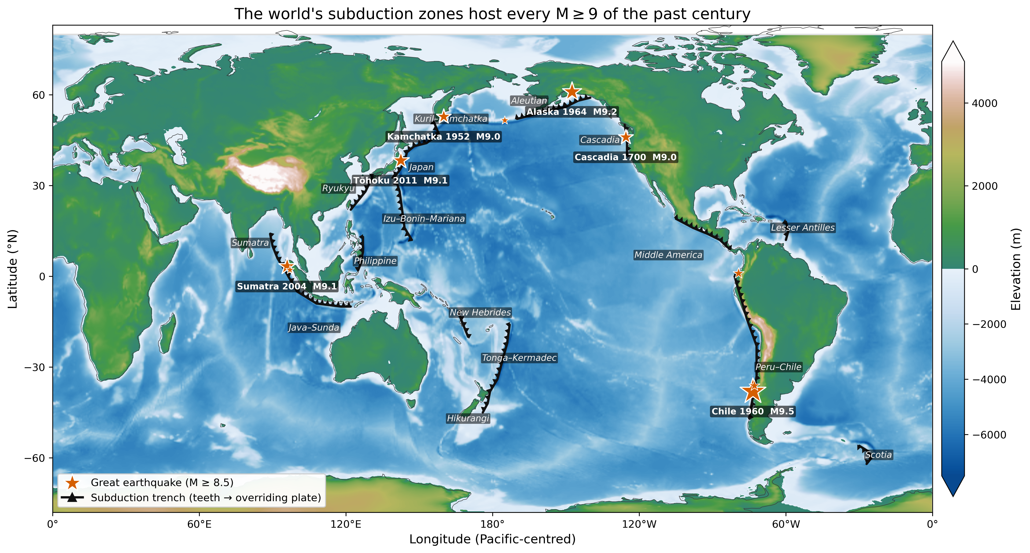— Fig. 154 The world’s subduction zones, with the great earthquakes ($M \geq 8.5$) of the past century. The trenches form the Pacific “Ring of Fire” together with the Sunda, Tethyan, and Caribbean–Scotia systems. Every $M\,9$ of the instrumental era occurred on a subduction megathrust — but those giants are spread across margins of widely differing plate age, convergence rate, and sediment supply, the first hint that the controlling parameters are not the obvious ones. Trench geometry after Hayes *et al.* [2018] (Slab2); great-earthquake locations from the USGS/Global CMT catalogues as summarised by Wirth *et al.* [2022]. Produced by `assets/scripts/fig_28_global_trenches.py`.#

The framing question for the lecture is therefore not “where do subduction earthquakes occur” — Fig. 154 answers that — but:

What physical properties of a subduction zone control how it deforms, how it fails, and how large an earthquake and tsunami it can produce — and why did the parameters everyone first reached for turn out to be the wrong ones?

The answer organizes the rest of the lecture. The classification that failed is worth teaching precisely because it failed: it is a clean example of how a physically reasonable hypothesis is revised against data, and it leads directly to the controls the modern literature does favour.

1a. Orientation: the anatomy of a subduction zone#

Before developing the physics, we need a shared visual vocabulary. The block diagram below (Fig. 155) labels the nine structural domains that will appear in every section of this lecture. Read through the labels once now — not to memorize them, but to map the words onto a geometry. Each label will be invoked again, with its physics, in §2–§10.

Three-dimensional perspective block diagram of an ocean-to-continent subduction zone. Oceanic lithosphere at the lower left, labeled A, bears prominent horizontal seafloor-spreading lineations and moves toward the continent (arrow pointing lower right). Nine structural domains are labeled in red. Along the top surface from left to right: A, oceanic lithosphere with spreading lineations; B, the deep-sea trench, the surface trace of the subduction hinge; C, the accretionary prism, a wedge of deformed and stacked sediments immediately landward of the trench; D, the forearc basin, a sediment-filled depression between the prism and the arc; E, the volcanic arc, shown as a broad highland with a prominent stratovolcano; F, the back-arc region, rugged mountainous terrain representing shortening on a Chilean-type margin; G, the continental interior on the far right. Below the surface, the thick black inclined slab (label I) descends from the trench beneath the overriding plate; vertical wavy lines at label H, beneath the volcanic arc, represent hot mantle and slab-derived fluids rising into the mantle wedge. The word OCEANIC LITHOSPHERE labels the left side; CONTINENTAL LITHOSPHERE labels the right side. 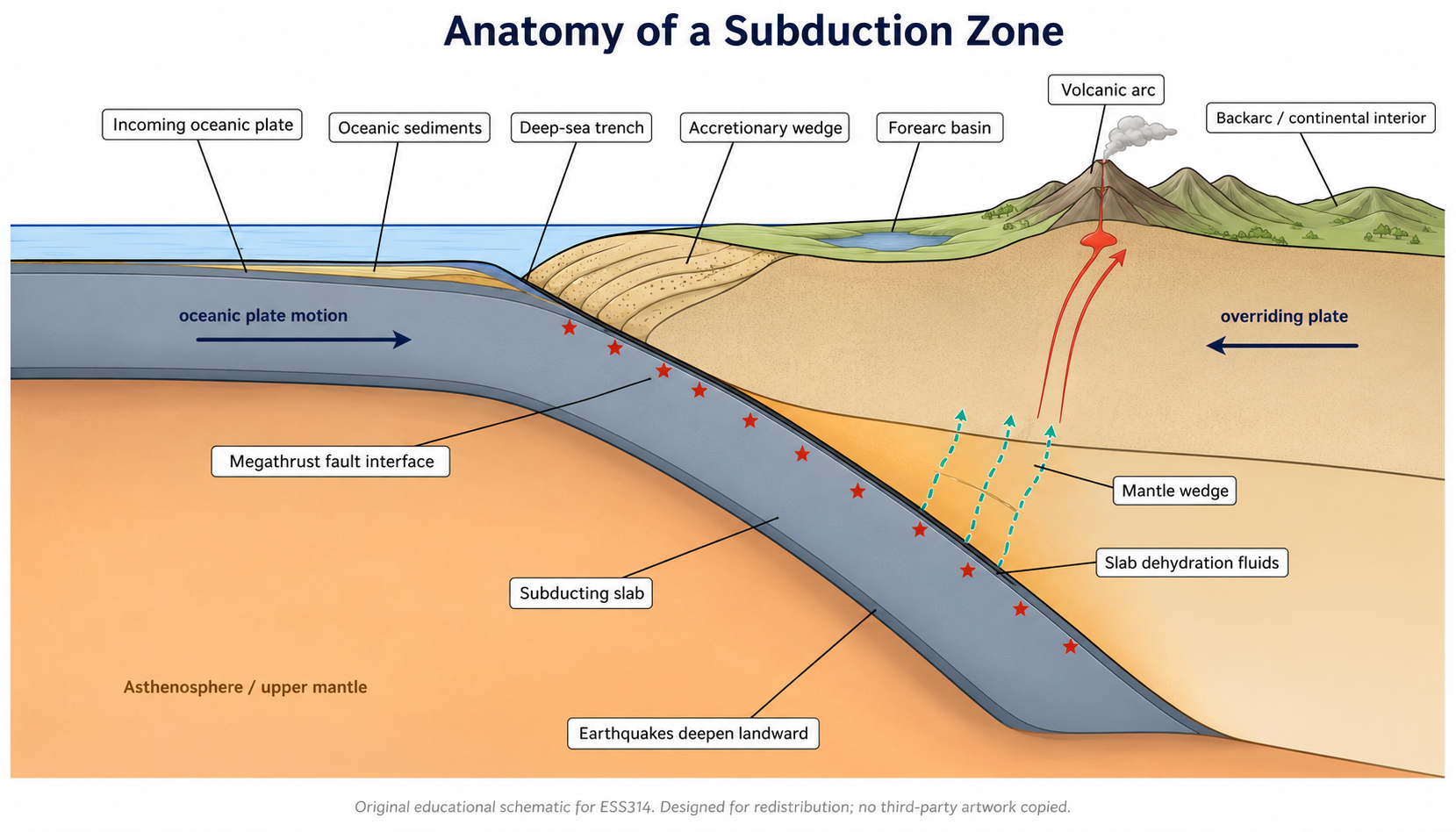— Fig. 155 **Road map for Lecture 28.** Nine labeled domains of an ocean–continent subduction zone. The oceanic plate (left, A) approaches the trench (B), where the denser slab (I) begins its descent. Scraped-off sediments pile into the accretionary prism (C); the forearc basin (D) sits between the prism and the volcanic arc (E). Slab dehydration releases fluids (H) that trigger partial melting in the mantle wedge and feed the arc volcanoes. The back-arc (F) and continental interior (G) record the stress state of the overriding plate. Every equation and hazard discussed in §2–§10 can be located on this figure. This figure is also used on the L28 quiz — see §11 for the identification table.#

The story of a subduction zone, read left to right through the labels, is a story of heat and water. Cold, dense oceanic lithosphere (A) arrives at the trench (B) and sinks along the megathrust (I). As it descends it cools the surrounding mantle and releases water from hydrous minerals (H). That water lowers the melting point of the overlying mantle wedge, generating magma that rises to build the volcanic arc (E). The stress transmitted across the interface determines whether the overriding plate shortens — building mountains in the back-arc (F) as at the Andes — or extends, opening a back-arc basin as in the western Pacific. Every measurable parameter that matters for earthquake hazard is a proxy for how efficiently this system transfers heat and how strongly the two plates grip each other at I.

2. Governing Physics#

2.1 The slab as a cold, dense sinker#

A subducting slab is oceanic lithosphere that has cooled and thickened away from its ridge (L26 §2). By the time it reaches a trench it is colder, and therefore denser, than the asthenosphere beneath it. That negative buoyancy is the engine of subduction: the weight of the sinking slab (label I in quiz4_cartoon) pulls the trailing plate along behind it. Slab pull is generally regarded as the dominant force in the plate-tectonic budget, larger than the ridge push that drives plates away from spreading centres.

The density contrast that drives the slab down has two parts, exactly as in the lithosphere comparison of L26 §6.1. The thermal contrast comes from the slab being colder than its surroundings; it grows with the age of the incoming plate (label A), because older lithosphere is thicker and colder. The compositional contrast comes from the basalt-to-eclogite transition: as the basaltic oceanic crust descends and increases in pressure, it transforms to eclogite, a denser assemblage that adds to the slab’s negative buoyancy. Both effects make an old slab a more vigorous sinker than a young one — which is exactly why the original Ruff–Kanamori reasoning was physically appealing.

2.2 Coupling on the megathrust#

The boundary between the descending slab (I) and the overriding plate (G) is the megathrust — the largest fault surface on Earth, and the source of every great subduction earthquake. Its surface trace at the seafloor is the trench (B).

Its behaviour is governed by how strongly the two plates are mechanically locked, or coupled, across the interface.

Where the megathrust is strongly coupled, the plates lock during the interseismic period, strain accumulates in the overriding plate, and that strain is released suddenly in great earthquakes. Where the megathrust is weakly coupled, the plates slide past one another more aseismically, and little strain accumulates to be released seismically. The degree of coupling is not a fixed property of a margin; it varies with depth along the interface and along strike, and it depends on temperature, fluid pressure (derived in part from slab dehydration at H), and the physical state of the material caught in the fault zone.

2.3 Two end-member modes#

Uyeda and Kanamori [1979] recognized that subduction zones occupy a continuum between two dynamic end-members, anchored by the contrast between the Chilean and Mariana margins (Fig. 156).

Two cross-section schematics side by side. Left, Chilean type: a young buoyant slab subducts at a shallow ~25 degree angle, strongly coupled to the overriding plate, with the volcanic arc far from the trench, and orange arrows showing back-arc shortening; labeled strong coupling leading to M9. Right, Mariana type: an old dense slab sinks steeply at ~70 degrees, weakly coupled, with the arc close to the trench, and green arrows showing back-arc extension; labeled weak coupling leading to no great earthquakes. 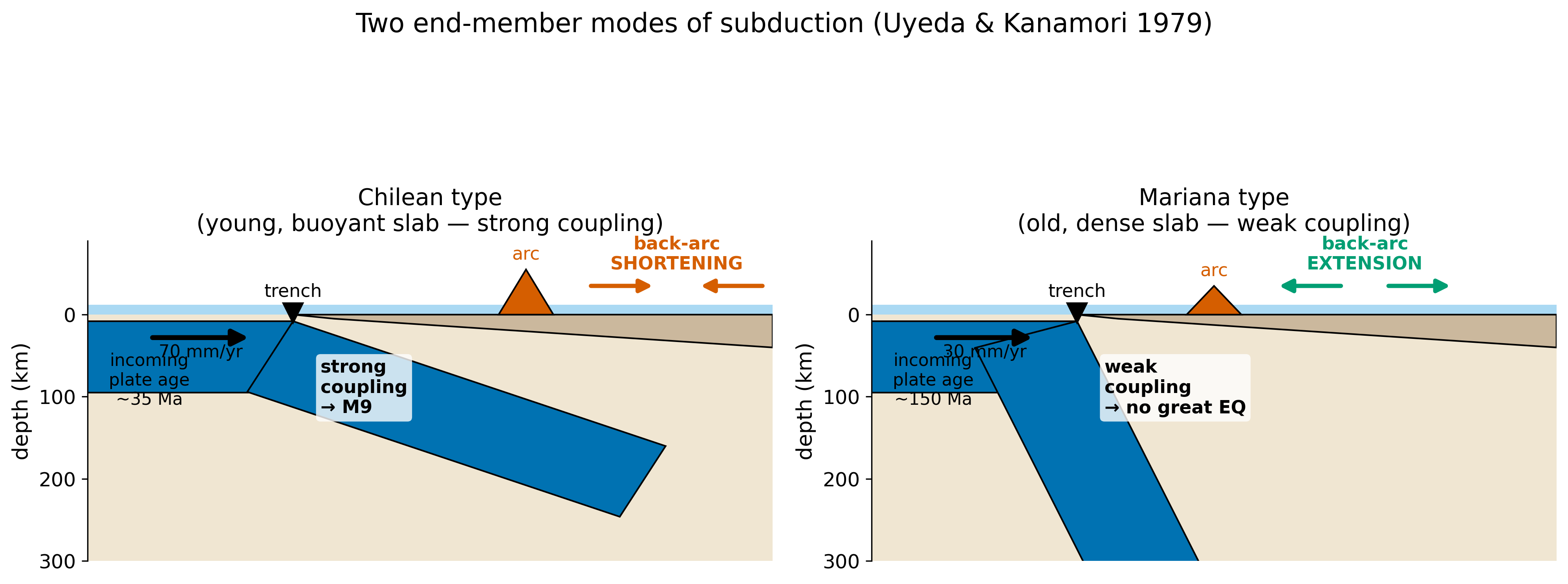— Fig. 156 The two end-member modes of subduction [Uyeda and Kanamori, 1979]. **(left) Chilean type:** a young, buoyant slab resists sinking and subducts at a shallow angle; it presses against the overriding plate (strong coupling), driving back-arc shortening and building a high mountain arc, and it hosts great ($M\,9$) earthquakes. **(right) Mariana type:** an old, dense slab sinks steeply and rolls back; coupling is weak, the trench retreats, and the back-arc is pulled into extension (active back-arc spreading). Mariana-type margins produce frequent small-to-moderate earthquakes but no recorded great events. Real margins lie on a continuum between these idealizations.#

The Chilean end-member has a young, buoyant slab (I), a shallow dip, strong coupling, back-arc shortening — building the Andes (F) — and great earthquakes. The accretionary prism (C) is thick at sediment-rich Chilean-type margins. The Mariana end-member has an old, dense slab (I), a steep dip, weak coupling, trench rollback, and back-arc extension (active spreading in the Mariana Trough, where F opens rather than compresses); the prism (C) is thin or absent. The continuum between them was the first physically grounded dynamic classification of convergent margins, and it remains a useful organizing idea. Its limitation — which the next two sections develop — is that the simple “old/dense/coupled → big earthquakes” expectation does not survive contact with the global earthquake record.

2.4 Intra-oceanic versus ocean–continent subduction#

The Chilean–Mariana continuum tracks a second, more concrete distinction: the nature of the overriding plate. Only oceanic lithosphere subducts readily, so the subducting plate is oceanic in every case; what differs is what sits above it.

In intra-oceanic (ocean–ocean) subduction, the overriding plate is also oceanic — thin, dense, and mechanically weak. These margins tend toward the Mariana end-member: a steep slab, weak coupling, trench rollback, and back-arc spreading, with volcanic island arcs built on oceanic crust (the Mariana, Tonga–Kermadec, Izu–Bonin, and Lesser Antilles arcs). In ocean–continent subduction, the overriding plate is continental — thick, buoyant, and strong — and the margin tends toward the Chilean end-member: a shallower slab, stronger coupling, back-arc shortening, and tall continental (Andean-type) arcs whose magmas are more evolved from their passage through thick crust (the Andes, Cascadia, Sumatra). The overriding-plate type therefore sets arc character, the style of back-arc deformation, and — through coupling — much of the great-earthquake behaviour. It is also the first step of the broader spectrum taken up in §5: an ocean–continent margin is what a subduction zone becomes just before its ocean runs out.

3. Mathematical Framework#

3.1 Notation#

Notation

Symbol	Meaning	Typical value / units
$A$	Age of incoming plate at the trench	$0$–$170$ Ma
$v_c$	Convergence rate (trench-normal)	$0$–$240$ mm/yr
$\delta$	Slab dip (deep)	$10$–$80^\circ$
$\Phi$	Thermal parameter	km (defined below)
$h_s$	Trench sediment thickness	$0$–$4$ km
$W$	Seismogenic-zone downdip width	$50$–$200$ km
$L$	Along-strike rupture length	up to $\sim 1500$ km
$\bar{D}$	Average coseismic slip	m
$\mu$	Shear modulus of fault-zone rock	$\sim 30$–$50$ GPa
$M_0$	Seismic moment	N·m
$M_w$	Moment magnitude	dimensionless

A note on convergence rate

The subduction literature, and the classification figures of this lecture, report the trench-normal convergence rate in an absolute (hotspot, HS3-NUVEL1A) reference frame rather than the plate-pair relative rate defined kinematically in L26 §7.2. The two differ — sometimes greatly. The 2004 Sumatra–Andaman segment, for example, has a trench-normal absolute rate near $3$ mm/yr even though the Indian–Sunda plates approach at several centimetres per year, because much of that motion is oblique and the overriding plate is itself moving. The distinction matters when reading Fig. 157.

3.2 The thermal parameter#

The thermal state of a slab — how cold it remains as it descends — is what couples the three “classic” parameters into a single quantity. A slab stays colder if it is older when it arrives (more accumulated cooling), if it descends faster (less time to reabsorb heat at depth), and if it dips more steeply (it spends less horizontal distance warming up per unit depth). These combine into the thermal parameter

(207)#\[ \Phi = A \, v_c \, \sin\delta , \]

with $A$ the incoming-plate age, $v_c$ the convergence rate, and $\delta$ the dip. A large $\Phi$ describes a cold slab that penetrates deep before warming; a small $\Phi$ describes a warm slab that equilibrates shallow. The thermal parameter sets the depth of the deepest earthquakes in a slab and the position of the basalt–eclogite transition, and — through temperature-dependent friction — it influences where on the interface the megathrust can store elastic strain.

The thermal parameter is the quantitative heart of the classic expectation: large $\Phi$ (old, fast, steep) was supposed to mean strong coupling and great earthquakes. Keep (207) in mind; the following sections connect it to real margins.

3.3 Seismic moment and the geometry of rupture#

The size of an earthquake is its seismic moment,

(208)#\[ M_0 = \mu \, \bar{D} \, A_{\mathrm{rupture}} = \mu \, \bar{D} \, (L \, W), \]

the product of the shear modulus, the average slip, and the ruptured fault area, written here as along-strike length $L$ times downdip width $W$. Moment magnitude follows from the moment by the standard relation

(209)#\[ M_w = \tfrac{2}{3} \log_{10} M_0 - 6.07 \quad (M_0 \text{ in N·m}). \]

Equation (208) reframes the central question in a more useful way. The maximum magnitude a margin can produce is controlled by the maximum fault area it can rupture coseismically, multiplied by the slip that area can store. The downdip width $W$ is set by the geometry of the seismogenic zone — the depth range over which the interface is locked and able to store elastic strain — and the along-strike length $L$ is set by how far a rupture can propagate before it runs into a barrier. Neither $L$ nor $W$ is a simple function of plate age or convergence rate. This is the mathematical reason the classic recipe fails: maximum magnitude scales with seismogenic geometry, not with the slab’s thermal vigour.

Key Equation — what limits the largest earthquake

The maximum moment of a subduction zone is set by the largest area it can rupture and the slip that area can hold: $$ M_0^{\max} = \mu \, \bar{D}^{\max} \, L^{\max} \, W^{\max}. $$ A wide, long, strongly locked seismogenic zone produces great earthquakes regardless of whether the incoming plate is young or old, fast or slow. The controls on $L^{\max}$ and $W^{\max}$ — interface dip, temperature, sediment, and roughness — are the parameters the modern literature actually uses.

4. Worked Example: Classifying Three Margins#

The key empirical result motivating this exercise is that maximum earthquake magnitude correlates with the geometry of the seismogenic zone — not with plate age or convergence rate. Wirth et al. [2022] test this directly by comparing the maximum observed $M_w$ of well-constrained margin segments against eight subduction parameters (Fig. 157).

Four scatter panels of maximum moment magnitude versus a subduction parameter, after Wirth et al. 2022 Table 1 and Figure 3. Top row, the dispelled recipe: panel a, subducting-plate age, shows no correlation (Wirth r = 0.05) with the giant M ≥ 9 earthquakes (vermillion stars) scattered across all ages from Cascadia at 7 Ma to Tohoku at 132 Ma; panel b, trench-normal convergence rate in the HS3-NUVEL1A absolute frame, shows no correlation (r = 0.19) with Sumatra a giant at only 3 mm/yr. Bottom row, the geometric controls: panel c, seismogenic-zone width, shows the strongest correlation (r = 0.44) with every giant above 110 km width and dashed thresholds at 75 km (all M ≥ 8.5) and 150 km (all M ≥ 9.2); panel d, downdip curvature, shows the giants clustering at low curvature, the flatter-ruptures-larger result (|r| = 0.42, Bletery 2016). 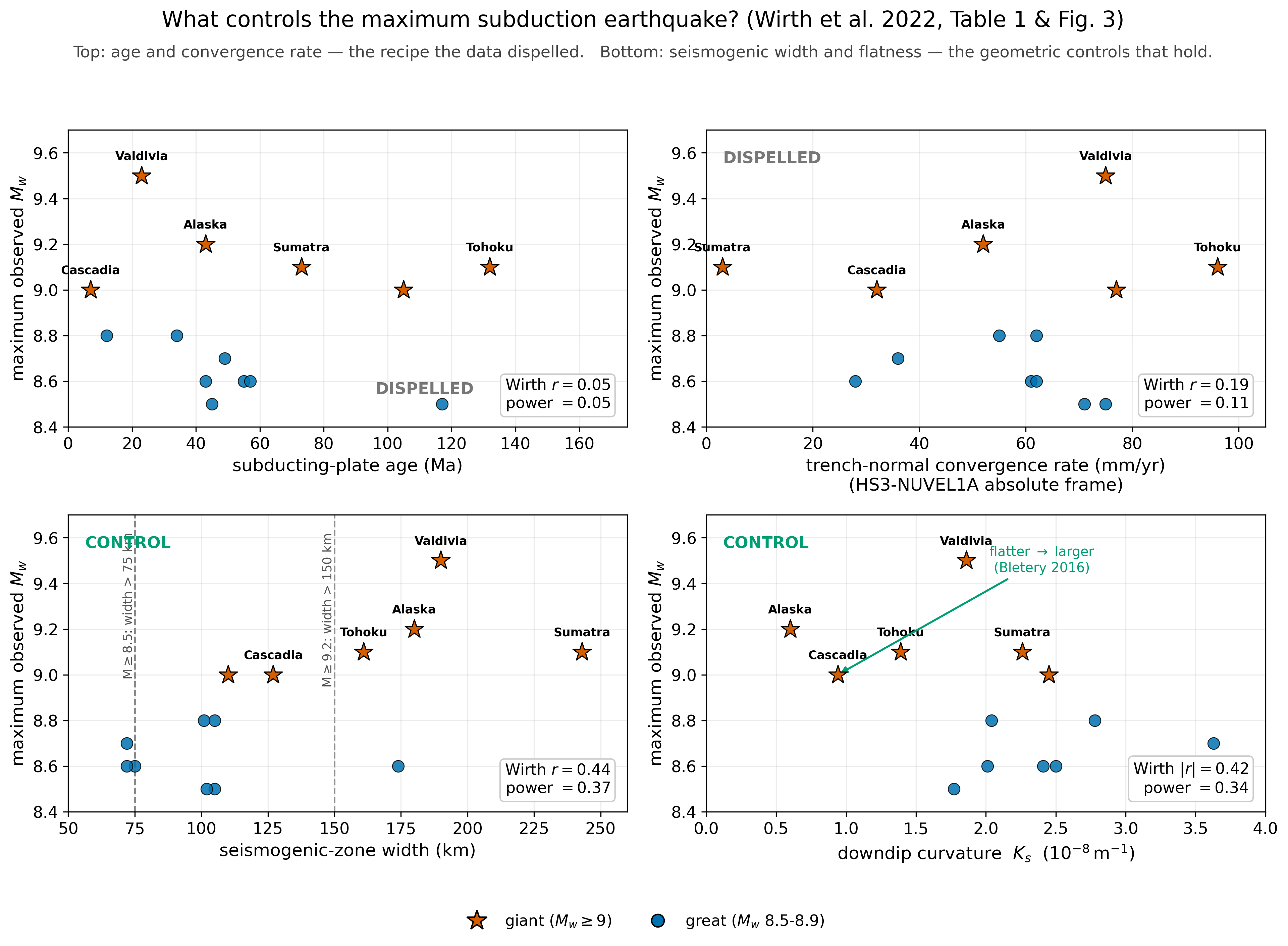— Fig. 157 Which parameter controls the maximum earthquake? Maximum observed $M_w$ against four subduction parameters for the well-constrained margin segments of Wirth *et al.* [2022], Table 1. **Top row — the recipe the data dispelled. (a)** Plate age: no correlation ($r = 0.05$). The giant ($M \geq 9$) earthquakes (stars) span the full age range — young Cascadia ($7$ Ma), old Tōhoku ($132$ Ma). **(b)** Trench-normal convergence rate: no correlation ($r = 0.19$). Sumatra–Andaman is a giant at a trench-normal rate of only $3$ mm/yr. **Bottom row — the geometric controls that hold. (c)** Seismogenic-zone width: the strongest single control ($r = 0.44$). Every giant has a width above $\sim 110$ km. **(d)** Downdip curvature: flatter megathrusts rupture larger ($|r| = 0.42$; Bletery *et al.* [2016]). Produced by `assets/scripts/fig_28_parameter_space.py`.#

The companion notebook notebooks/subduction_parameter_space.ipynb carries out the full quantitative classification interactively, loading the per-zone table behind Fig. 157 and letting the reader reposition any margin and test the correlation. The qualitative version of that exercise, worked here, compares three margins that occupy very different parts of the parameter space yet have all produced — or are expected to produce — great earthquakes.

Chile (Maule segment). Incoming plate $\sim 33$ Ma, converging fast ($\sim 68$ mm/yr) at a shallow dip; strongly coupled; back-arc shortening builds the Andes. This is the Chilean end-member of §2.3 — and it behaves as the classic recipe expects, hosting the 2010 $M\,8.8$ and the 1960 $M\,9.5$, the largest instrumentally recorded earthquake.

Mariana. Incoming plate very old ($\sim 155$ Ma) but converging slowly ($\sim 35$ mm/yr) at a steep dip; weakly coupled; back-arc extension opens the Mariana Trough. The classic recipe, weighting old age heavily, would have flagged this as a great-earthquake candidate. It is not: no great earthquake has been recorded here. The steep dip and weak coupling give it a narrow seismogenic width $W$, and (208) limits the moment accordingly.

Cascadia. Incoming plate young ($< 15$ Ma), converging slowly ($\sim 35$–$45$ mm/yr); warm slab; thick sediment; no bathymetric trench. By the classic recipe — young and slow — this is the least likely place for a great earthquake. Yet the paleoseismic record shows it produced an $M \sim 9$ in 1700, and it is the focus of §10.

The three margins make the lesson concrete: Chile fits the old recipe, Mariana breaks it in one direction (old but no great earthquakes), and Cascadia breaks it in the other (young but $M\,9$-capable). A classification scheme that cannot accommodate all three is not describing the controlling physics.

5. The Convergence Spectrum: From Subduction to Collision#

Subduction is the steady state of a convergent margin, but it is not the whole story. A subduction zone consumes oceanic lithosphere at the rate the plates converge, and oceanic lithosphere is finite. As an ocean closes, the material arriving at the trench becomes progressively more buoyant, and the margin moves along a spectrum from subduction toward collision (Fig. 158). The organizing principle is buoyancy: oceanic lithosphere is dense enough to subduct, but continental crust is too light to be carried deep into the mantle, so when continental material reaches the trench, subduction stalls and the convergence is taken up by deformation instead.

Four schematic cross-sections arranged two by two showing the spectrum of convergent margins. Panel a, intra-oceanic subduction, has an oceanic plate subducting steeply beneath a thin oceanic upper plate with a volcanic island arc and back-arc spreading (Mariana, Tonga). Panel b, ocean-continent subduction, has an oceanic plate subducting at shallower angle beneath a thick continental plate with a tall Andean arc and back-arc shortening (Andes, Cascadia). Panel c, arc-continent collision, shows a buoyant continental margin arriving at the trench and a volcanic arc colliding with it to build a rising doubly-vergent orogen (Taiwan). Panel d, continent-continent collision, shows two continental plates with one underthrusting the other along a detachment megathrust, thickening the crust into a plateau (Himalaya-Tibet, Arabia-Zagros). 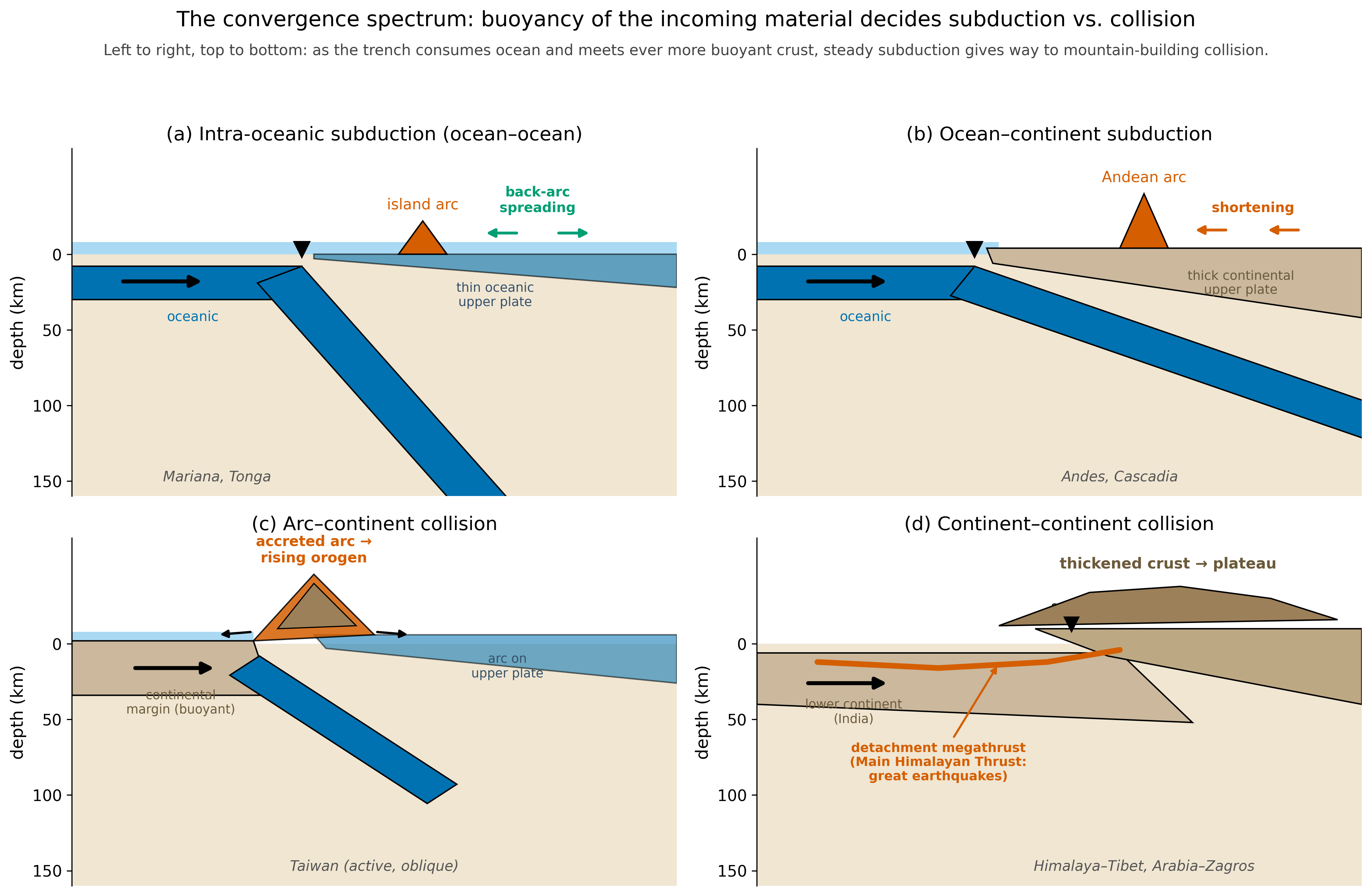— Fig. 158 The spectrum of convergent margins, ordered by the buoyancy of the incoming material. **(a)** Intra-oceanic subduction (§2.4): both plates oceanic, island arc, back-arc spreading. **(b)** Ocean–continent subduction: oceanic slab beneath a thick continental plate, Andean arc, back-arc shortening. **(c)** Arc–continent collision: a continental margin reaches the trench and its volcanic arc collides with it, raising a young orogen — Taiwan, where the collision is active today. **(d)** Continent–continent collision: buoyant continental crust resists subduction, so convergence thickens the crust along a detachment megathrust and raises a plateau. Produced by `assets/scripts/fig_28_convergence_spectrum.py`.#

Arc–continent collision is the spectrum’s midpoint and its clearest live example is Taiwan. There, the Luzon volcanic arc, riding the Philippine Sea plate, is colliding obliquely with the passive continental margin of the Eurasian plate. Because the collision is oblique it propagates southward, so a north-to-south traverse of the island is a snapshot of the process through time — incipient collision in the south, a mature doubly-vergent mountain belt in the centre, and post-collisional collapse in the north [Teng, 1990]. Taiwan also shows that subduction polarity can reverse across such a junction. The mountains rise fast, erosion is among the most rapid on Earth, and the collision-related thrusts are seismically dangerous: the 1999 $M\,7.6$ Chi-Chi earthquake ruptured one of them.

Continent–continent collision is the spectrum’s endpoint, reached when the ocean is entirely gone. The type example is the India–Eurasia collision that began roughly 50 million years ago and built the Himalaya and the Tibetan Plateau, where the crust has been thickened to nearly twice its normal value and the excess is partly accommodated by lateral extrusion of Asia eastward [Molnar and Tapponnier, 1975]. The Arabia–Eurasia collision is its younger cousin, raising the Zagros and the Caucasus. Collision does not switch off great earthquakes — it relocates them: India underthrusts Eurasia along the Main Himalayan Thrust, a continental detachment that behaves much like a megathrust and has produced great events including the 1934 $M\,8.0$ Bihar–Nepal earthquake and the 2015 $M\,7.8$ Gorkha earthquake [Avouac et al., 2015]. The seismic-moment reasoning of §3.3 applies here too: a wide, gently dipping detachment can store a large rupture area, so collisional megathrusts remain capable of great, damaging earthquakes even though no oceanic slab is being consumed.

The spectrum reframes this lecture’s subject. Subduction zones are the convergent margins that still have ocean to consume; collisional belts are what they become when the ocean is gone. The physics is continuous across the spectrum — buoyancy drives the descending plate, coupling and geometry govern the earthquakes — which is why the same toolkit carries from Cascadia to the Himalaya.

6. Course Connections#

Where this lecture connects

L26 §7 (Plate Boundaries and Relative Motion): This lecture is the convergent case of the kinematic classification. The convergence rate $v_c$ used throughout is the relative-velocity magnitude defined there; the Mendocino triple junction worked in L26 §7.4 places the northern end of the Cascadia margin, and the subduction-polarity point made there is why §2.1 must invoke buoyancy, not kinematics, to say which plate descends.
L04–L07 (Seismic waves): Wadati–Benioff seismicity is located by the travel-time methods developed there.
L13–L16 (Earthquake source): The megathrust is a thrust fault; its focal mechanism, moment (208), and magnitude (209) are the source quantities introduced there.
L16–L17 (Ground motions and tsunamis): The domain-based tsunami and strong-motion sources are the inputs to the hazard methods of those lectures.
L27 (Ridges and Rifts): The divergent counterpart — where the oceanic lithosphere that arrives at these trenches was born.
L29 (Transforms & Intraplate): The third boundary class, and the breakdown of the rigid-plate assumption that circuit closure (L26 §7.4) depends on. The distributed deformation of continental collision (§5) is an extreme case of that breakdown.
L30 (Plate Tectonics and Geodynamics): Slab pull (§2.1) is the dominant term in the global force and heat budget assembled in the capstone, and the convergence spectrum of §5 — from intra-oceanic subduction through continental collision — is the framework the capstone uses to read the rock record of closed oceans.

7. Research Horizon#

The study of great subduction earthquakes is in an unusually active phase, driven by the well-recorded giants of 2004, 2010, and 2011 and by new offshore instrumentation. Three open-access entry points:

Wirth et al. [2022], Nature Reviews Earth & Environment — the synthesis that frames this lecture. It documents the failure of the age/convergence-rate hypotheses and reviews the rupture characteristics (seaward and landward extent, strong-motion-generating areas, recurrence) that actually govern hazard. Open access through the USGS Publications Warehouse.
Lay and Nishenko [2022], PNAS — updates the concepts of seismic gaps and asperities along South America, where the long earthquake record makes it possible to ask how repeatable great ruptures are. A useful counterpoint to the “any margin can do it” conclusion: long-term plate-boundary strain budgets do impose a degree of cyclicity. Palaeoseismic archives — coral microatolls in Sumatra, turbidite sequences and drowned soils in Cascadia — reveal that recurrence is rarely simple: many margins show supercycles, clusters of differently sized ruptures separated by long quiet intervals, rather than clockwork repetition. The 2010 Maule earthquake filled a recognized seismic gap last ruptured in 1835. Open access.
Biemiller and others [2024], JGR Solid Earth — examines how megathrust geometry (dip and seismogenic width) shapes maximum magnitude and recurrence, part of the modern shift toward geometry-based controls.

Open research question

If essentially any mature megathrust can host an $M\,9$, what observable — geometry, sediment, fluid pressure, or something not yet identified — most sharply distinguishes the segments that will from those that will not? Offshore geodesy and seafloor seismology at Cascadia (§10) are being deployed to answer exactly this, and the answer will reshape hazard maps for the Pacific Northwest.

8. Societal Relevance: Cascadia, the M9-Capable “Exception”#

The Cascadia subduction zone runs offshore from northern California to southern British Columbia, directly west of every student reading this. The Juan de Fuca plate — born at the ridge of L26, young and warm by the time it reaches the margin — descends beneath North America at $\sim 35$–$45$ mm/yr (Fig. 159).

West-to-east cross-section of the Cascadia subduction zone. The young, warm Juan de Fuca plate (blue) moves east at 35-45 mm/yr and descends beneath North America. A thick orange sediment layer rides on the incoming plate; there is a buried deformation front with no bathymetric trench and a large accretionary wedge. The megathrust interface is marked as a locked seismogenic zone (the 1700 M9 rupture) updip and an episodic-tremor-and-slip zone downdip, with the Cascade arc volcano to the east. A call-out box notes that Cascadia is young, slow, sediment-rich, and smooth — the opposite of the old big-earthquake recipe — yet is M9-capable. 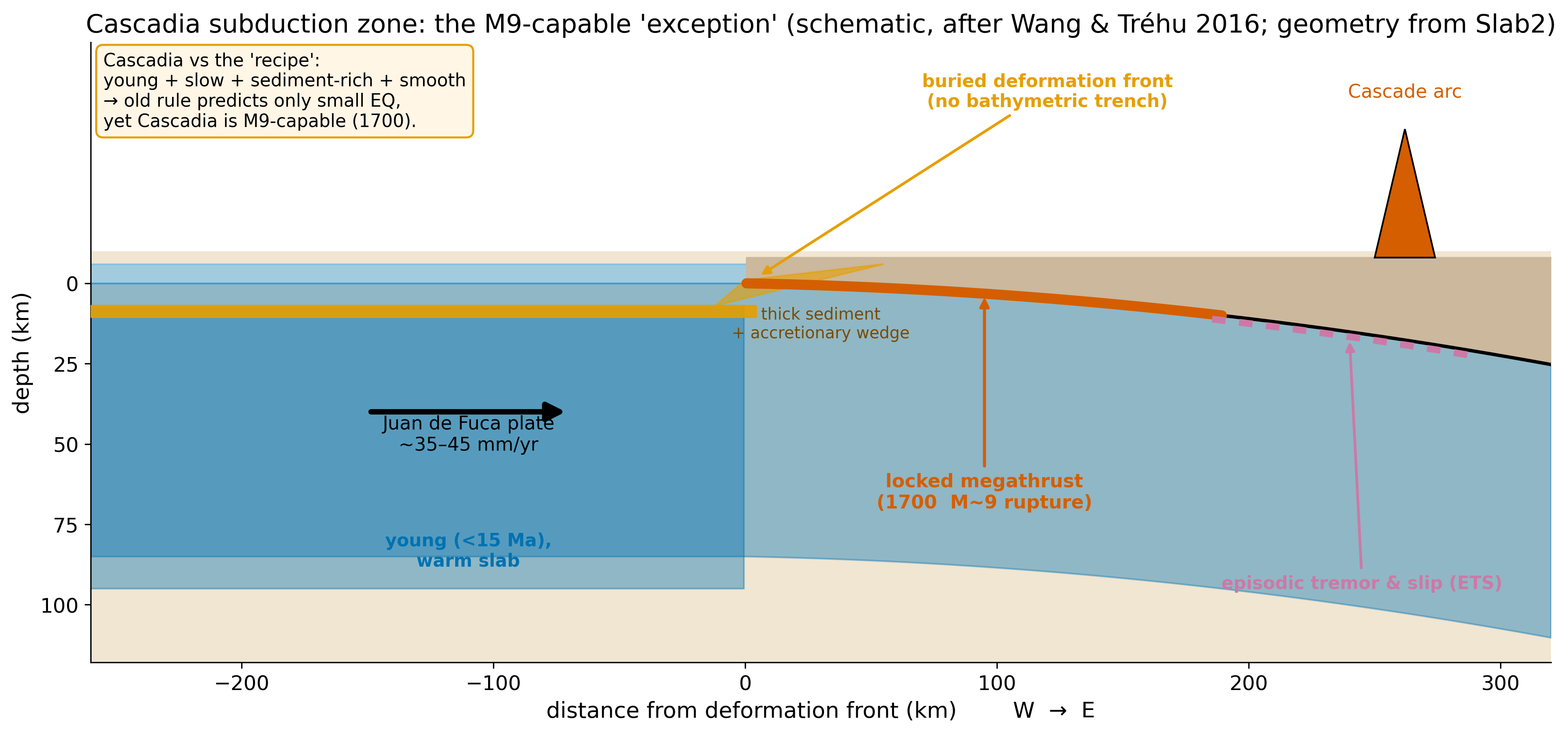— Fig. 159 Cascadia subduction zone cross-section: the $M\,9$-capable “exception.” The young ($< 15$ Ma), warm Juan de Fuca slab, the slow convergence, the thick incoming sediment, the buried deformation front with no bathymetric trench, and the unusually smooth interface are every ingredient the classic recipe says should produce only modest earthquakes. The paleoseismic record says otherwise: the megathrust is locked, and it produced an $M \sim 9$ in January 1700. Episodic tremor and slip (ETS) occupies the deep transition zone. Schematic after Wang and Tréhu [2016]; geometry consistent with Slab2 [Hayes *et al.*, 2018]. Produced by `assets/scripts/fig_28_cascadia_section.py`.#

By the parameters of the classic recipe — young, slow — Cascadia is the last place one would expect a great earthquake. By the modern controls it is one of the most concerning margins on Earth. Its geometry alone places it firmly in great-earthquake territory: Wirth et al. [2022] give it a seismogenic width of $127$ km and a shallow interface dip of $11^\circ$ — comfortably past the $>75$ km / $<35^\circ$ threshold for $M \geq 8.5$, and a smooth, near-planar megathrust. The thick, well-consolidated sediment smooths the interface further and may allow rupture to propagate the full $\sim 1000$ km length of the margin and breach the trench, the two ingredients (large $L$, shallow domain-A slip) that produce a long, strongly tsunamigenic rupture [Han et al., 2017, Wang and Tréhu, 2016]. The evidence that this has happened is unambiguous: the January 1700 earthquake is dated to the night of 26 January 1700 by the tsunami it sent across the Pacific to Japan [Satake et al., 2003], and recorded along the Cascadia margin by drowned forests and by the offshore turbidites it shook loose.

The practical message for a Pacific Northwest resident in 2026 is the lecture’s thesis made local. The framework that says “old and fast means dangerous” would have rated Cascadia low. The framework built in this lecture — maximum magnitude set by seismogenic geometry and interface smoothness, not by slab age — rates it among the most hazardous, capable of an $M\,9$ megathrust earthquake and an accompanying near-field tsunami with little warning. The classification that data dispelled was not an academic curiosity; getting it wrong would mean preparing for the wrong earthquake.

AI Literacy: Epistemics — Catching the Confident, Outdated Answer#

AI Prompt Lab — what controls the maximum earthquake size?

A prompt to try with an AI assistant:

What controls the maximum earthquake magnitude a subduction zone can produce? Explain how plate age and convergence rate determine the largest possible earthquake.

Notice that the prompt itself contains the obsolete assumption — that age and rate are the controls. A capable assistant may accept the premise and produce a fluent, confident explanation of the Ruff–Kanamori relationship, complete with the physical reasoning of §2.1, and never mention that the hypothesis was dispelled by the 2004 and 2011 earthquakes.

Your task: grade the response against the rubric below.

Criterion	Pass	Fail
Does the response challenge the premise of the question?	flags that age/rate do not control $M_{\max}$	accepts the premise uncritically
Does it cite the falsifying evidence?	names Sumatra 2004 and/or Tōhoku 2011	presents the 1980 recipe as current
Does it give the modern controls?	seismogenic geometry, smoothness/sediment, fluids	offers only age and rate
Is it appropriately uncertain?	notes that any mature megathrust may be $M\,9$-capable	states a confident, deterministic rule

This is the most important AI-literacy exercise in Module 7, because it is the failure mode you are least likely to catch: the answer is fluent, internally consistent, physically reasonable, and wrong only because the science moved. An assistant trained on decades of literature will have seen the dispelled hypothesis stated as fact thousands of times. The defence is not better prompting — it is domain knowledge. You catch this error because you read Fig. 157, not because the AI flagged it. The lesson of the lecture and the lesson of the prompt lab are the same: a confident, well-formed explanation can encode a hypothesis the data have already overturned.

9. Concept Checks#

9a. Anatomy of a subduction zone#

The illustrated cross-section below (Fig. 160) uses plain-English text labels for every structural element of a subduction zone. Each text label corresponds directly to the letter callout (A–I) introduced in the road-map cartoon of §1a (quiz4_cartoon); the table that follows lists both names together so you can move fluently between the two representations. For each element, know its name, the dominant process it hosts, and how it connects to a hazard or equation from §2–§4.

Illustrated cross-section titled "Anatomy of a Subduction Zone." The oceanic plate (quiz4_cartoon label A) approaches from the left with a blue rightward arrow labelled "oceanic plate motion"; a thin layer of oceanic sediments rides on top. At the bend where the plate begins to descend, the deep-sea trench (B) forms the topographic low. Immediately landward, imbricate wedges of stacked sediment build the accretionary wedge (C). Behind it, a water-filled low forms the forearc basin (D). Further landward, a large erupting stratovolcano represents the volcanic arc (E), with a solid red arrow showing melt rising from depth through the overriding plate. To the right, green highland terrain marks the backarc and continental interior (F and G combined); a blue leftward arrow labelled "overriding plate" shows its motion. Below the surface, the thick grey descending slab (I, labelled "Subducting slab") dips from upper-left to lower-right. The slab-overriding-plate contact, labelled "Megathrust fault interface," is traced by a chain of red stars whose depth increases landward, with the annotation "Earthquakes deepen landward" — the Wadati–Benioff zone. From the slab surface, three cyan dashed arrows labelled "Slab dehydration fluids" (H) rise into the overlying "Mantle wedge" (H); the solid red magma arrows continue from the mantle wedge up to the volcanic arc. The warm tan-orange lower region is labelled "Asthenosphere / upper mantle." Footer: "Original educational schematic for ESS 314. Designed for redistribution; no third-party artwork copied." — Fig. 160 **Anatomy of a subduction zone** — the same nine domains introduced as labels **A–I** in the §1a road-map (`quiz4_cartoon`), now shown in a rendered cross-section with plain-English callouts. *Incoming oceanic plate* = A; *Oceanic sediments* = the sediment blanket on A; *Deep-sea trench* = B; *Accretionary wedge* = C; *Forearc basin* = D; *Volcanic arc* = E; *Backarc / continental interior* = F + G; *Slab dehydration fluids* + *Mantle wedge* = H; *Megathrust fault interface* + *Subducting slab* = I. Red stars trace the Wadati–Benioff zone deepening landward; cyan dashed arrows are the slab-fluid pathway that triggers arc volcanism; solid red arrows are rising melt. Original educational schematic for ESS 314.#

Label (§1a cartoon)	Figure text label (SF7)	Dominant process / hazard connection
A	Incoming oceanic plate / Oceanic sediments	Born at a mid-ocean ridge (L27); cooling thickens it and increases negative buoyancy (§2.1); age here sets the thermal parameter $\Phi$
B	Deep-sea trench	Surface trace of the subducting slab; deepest ocean floor; marks the updip end of the megathrust — if rupture reaches the trench, seafloor uplift generates a large tsunami
C	Accretionary wedge	Incoming sediments scraped off the oceanic plate and stacked against the overriding margin; thick at Cascadia, thin or absent at Mariana; a thick prism smooths the interface and may allow rupture to propagate along strike
D	Forearc basin	Sediment-filled basin between the prism and the volcanic arc; subsides during interseismic locking and may uplift coseismically; records the earthquake cycle stratigraphically
E	Volcanic arc	Chain of arc volcanoes produced by partial melting of the mantle wedge (H); the subareal expression of slab dehydration; position relative to the trench reflects slab dip
F	Backarc / continental interior (rear portion)	Compressional (shortening → Andes) on Chilean-type margins; extensional (rifting / back-arc spreading) on Mariana-type margins (§2.3)
G	Backarc / continental interior (craton) / overriding plate	Buoyant, thick, felsic; this positive buoyancy is why it overrides the denser oceanic slab (L26 §6); the overriding plate stores elastic strain during interseismic locking
H	Slab dehydration fluids + Mantle wedge	Water released by mineral dehydration in the descending slab lowers the peridotite solidus → partial melt rises to feed arc volcanoes at E; hydrous fluids also lower friction on the megathrust at I
I	Megathrust fault interface + Subducting slab	The subduction-interface fault — the largest fault on Earth; locking here stores the elastic strain released in $M\,8$–$9$ earthquakes; all great-subduction-zone earthquakes occur on this surface

Quiz-preparation questions

Practice answering each in 2–4 sentences. These are the styles of questions on the L28 quiz.

Part 1 — Label identification and process

Label I is called the megathrust. (a) What type of faulting mechanism does it have (thrust, normal, or strike-slip)? (b) What determines the depth at which earthquakes on I stop occurring (the base of the seismogenic zone)? (c) Name the two primary hazards generated when I ruptures to the trench (B).
Trace the process chain A → I → H → E: starting from the composition of the incoming oceanic crust at A, explain step by step how subduction ultimately produces a volcano at E.
The wavy lines at H represent fluid released from the slab. In what mineral reactions does this fluid originate? At roughly what depth? Why does the presence of this fluid lower the melting point of the overlying mantle?

Part 2 — Margin classification (§2.3)

In this diagram, label F shows a volcanic mountain range (like the Andes) behind the arc. Does this indicate a Chilean-type or Mariana-type margin? What does it imply about: (a) slab dip at I, (b) the degree of coupling, and (c) the expected maximum earthquake magnitude?
Redraw the diagram schematically for a Mariana-type margin. What happens to the trench (B), the accretionary wedge (C), and the back-arc (F)? What happens to the width of the seismogenic zone on I?

Part 3 — Hazard and seismic moment

The 2011 Tōhoku earthquake produced tens of metres of slip near B (the trench). Using the equation $M_0 = \mu \bar{D}\,L\,W$ ((208)): which term ($\bar{D}$, $L$, or $W$) was unexpectedly large, and why did conventional hazard models fail to anticipate it?

Part 4 — Cascadia application (§8)

At Cascadia, the bathymetric trench (B) is buried and the accretionary prism (C) is unusually thick.
- (a) What does a thick prism at C imply for the roughness of the interface at I?
- (b) How does a smooth interface affect the along-strike rupture length $L$ in (208)?
- (c) What additional control — related to the composition of sediment at C — does Han et al. [2017] identify as varying along strike?
Two students argue about the maximum earthquake Cascadia can produce. Student A says: “The incoming plate at A is young ($< 15$ Ma), so the slab is warm and buoyant; coupling should be weak and the maximum event moderate.” Student B says: “The thick, smooth sediment at C allows the full 1 000 km margin to rupture in a single event.” (a) Which student’s reasoning is consistent with Wirth et al. [2022]? (b) Which parameter in (208) is each student focusing on?

Part 5 — Cross-cutting synthesis

The figure shows a single snapshot of the subduction system. Describe what the same cross-section will look like in 10 million years: which label shrinks, which grows, and what tectonic event eventually terminates subduction at this margin?

A note on sensitive content

This lecture discusses earthquake and tsunami hazards that have caused large loss of life, including events within living memory. The intent is scientific and preparedness-oriented. Students in the Pacific Northwest who find the Cascadia hazard distressing may find it helpful to channel that concern into preparedness resources from the Washington Emergency Management Division and the Pacific Northwest Seismic Network.

[1]

Jean-Philippe Avouac, Lingsen Meng, Shengji Wei, Teng Wang, and Jean-Paul Ampuero. Lower edge of locked Main Himalayan Thrust unzipped by the 2015 Gorkha earthquake. Nature Geoscience, 8:708–711, 2015. doi:10.1038/ngeo2518.

[2]

James Biemiller and others. Megathrust geometry controls on maximum magnitude and recurrence of great subduction earthquakes. Journal of Geophysical Research: Solid Earth, 2024. doi:10.1029/2024JB029191.

[3]

Quentin Bletery, Amanda M. Thomas, Alan W. Rempel, Leif Karlstrom, Anthony Sladen, and Louis De Barros. Mega-earthquakes rupture flat megathrusts. Science, 354(6315):1027–1031, 2016. doi:10.1126/science.aag0482.

[4] (1,2)

Shuoshuo Han, Nathan L. Bangs, Suzanne M. Carbotte, Demian M. Saffer, and James C. Gibson. Links between sediment consolidation and cascadia megathrust slip behaviour. Nature Geoscience, 10:954–959, 2017. doi:10.1038/s41561-017-0007-2.

[5] (1,2)

Gavin P. Hayes, Ginevra L. Moore, Daniel E. Portner, Mike Hearne, Hanna Flamme, Maria Furtney, and Gregory M. Smoczyk. Slab2, a comprehensive subduction zone geometry model. Science, 362(6410):58–61, 2018. doi:10.1126/science.aat4723.

[6]

Thorne Lay and Stuart P. Nishenko. Updated concepts of seismic gaps and asperities to assess great earthquake hazard along South America. Proceedings of the National Academy of Sciences, 119(51):e2216843119, 2022. doi:10.1073/pnas.2216843119.

[7]

Peter Molnar and Paul Tapponnier. Cenozoic tectonics of Asia: effects of a continental collision. Science, 189(4201):419–426, 1975. doi:10.1126/science.189.4201.419.

[8]

Larry Ruff and Hiroo Kanamori. Seismicity and the subduction process. Physics of the Earth and Planetary Interiors, 23(3):240–252, 1980. doi:10.1016/0031-9201(80)90117-X.

[9]

Kenji Satake, Kelin Wang, and Brian F. Atwater. Fault slip and seismic moment of the 1700 Cascadia earthquake inferred from Japanese tsunami descriptions. Journal of Geophysical Research: Solid Earth, 108(B11):2535, 2003. doi:10.1029/2003JB002521.

[10]

Louis S. Teng. Geotectonic evolution of late Cenozoic arc–continent collision in Taiwan. Tectonophysics, 183(1–4):57–76, 1990. doi:10.1016/0040-1951(90)90188-E.

[11] (1,2)

Seiya Uyeda and Hiroo Kanamori. Back-arc opening and the mode of subduction. Journal of Geophysical Research: Solid Earth, 84(B3):1049–1061, 1979. doi:10.1029/JB084iB03p01049.

[12] (1,2)

Kelin Wang and Anne M. Tréhu. Invited review paper: some outstanding issues in the study of great megathrust earthquakes – the Cascadia example. Journal of Geodynamics, 98:1–18, 2016. doi:10.1016/j.jog.2016.03.010.

[13] (1,2,3,4,5,6,7)

Erin A. Wirth, Valerie J. Sahakian, Laura M. Wallace, and Daniel Melnick. The occurrence and hazards of great subduction zone earthquakes. Nature Reviews Earth & Environment, 3:125–140, 2022. doi:10.1038/s43017-021-00245-w.

Symbol	Meaning	Typical value / units
\(A\)	Age of incoming plate at the trench	\(0\)–\(170\) Ma
\(v_c\)	Convergence rate (trench-normal)	\(0\)–\(240\) mm/yr
\(\delta\)	Slab dip (deep)	\(10\)–\(80^\circ\)
\(\Phi\)	Thermal parameter	km (defined below)
\(h_s\)	Trench sediment thickness	\(0\)–\(4\) km
\(W\)	Seismogenic-zone downdip width	\(50\)–\(200\) km
\(L\)	Along-strike rupture length	up to \(\sim 1500\) km
\(\bar{D}\)	Average coseismic slip	m
\(\mu\)	Shear modulus of fault-zone rock	\(\sim 30\)–\(50\) GPa
\(M_0\)	Seismic moment	N·m
\(M_w\)	Moment magnitude	dimensionless