Seismic Refraction II — Beyond the Flat Layer

Seismic Refraction II — Beyond the Flat Layer#

Prerequisites#

Students should be comfortable with: the critical angle condition and derivation of the single-layer head-wave travel-time equation (\(t = x/V_2 + 2h_1\cos\theta_{ic}/V_1\)); Snell’s law in vector and scalar form; the concept of apparent velocity; and basic Python array operations.

1. The Geoscientific Question#

The refraction surveys described in Lecture 6 assumed the simplest possible Earth: a single horizontal layer overlying a faster half-space. Real near-surface geology is far more complex. The Cascadia forearc, the glacially reworked lowlands of the Puget Sound region, the Columbia River Basalt province — all present geologists and engineers with subsurface architectures that include multiple distinct velocity units, layers that thin laterally, interfaces that dip, and zones where velocity decreases with depth. Each of these configurations leaves a distinctive signature in the \(T\)-\(x\) diagram, and each produces a different class of interpretive ambiguity.

The motivating question is therefore two-fold. First, can the analytical framework developed for the single-layer case be extended systematically to more realistic Earth models? Second — and crucially — what are the limits of that framework? When refraction surveying is used to site a dam foundation, assess liquefaction potential, or map the depth to bedrock beneath a future highway corridor, the cost of misinterpreting a low-velocity zone or a hidden thin layer is not merely academic. Understanding model non-uniqueness and data uncertainty is as important as knowing the forward solution.

This lecture develops the generalized travel-time equations for multi-layer models, derives the dipping-interface solution from first principles, exposes the diagnostic failure modes of refraction analysis (the low-velocity zone problem, the thin-layer problem), and introduces the delay-time method for mapping irregular refractors. Throughout, sources of data uncertainty and their propagation into depth estimates are made explicit.

2. Governing Physics#

2.1 The Head Wave as a Boundary-Traveling Disturbance#

A head wave, or refracted wave, exists because at the critical angle \(\theta_{ic} = \sin^{-1}(V_1/V_2)\) the refracted ray travels along the interface at velocity \(V_2 > V_1\). This boundary-constrained propagation continuously re-radiates energy upward into the slower upper medium at the same critical angle. The physical mechanism is analogous to the Mach cone produced by a supersonic body: the refractor surface acts as a secondary source, and interference among secondary wavelets constructively reinforces the upward-going critically refracted wavefront.

Key Physical Insight

The head wave exists only when \(V_2 > V_1\). If the lower medium is slower than the upper medium (\(V_2 < V_1\)), no critical angle exists, and no head wave is generated at that interface. This is the physical basis of the low-velocity zone problem developed in Section 3.1.

2.2 The \(N\)-Layer Generalization#

For a horizontally layered model with \(N\) layers, the travel-time for the head wave refracted along the \(n\)-th interface (\(n \geq 2\), with the refractor velocity \(V_n\)) is obtained by summing the slant-path transit times through each overlying layer and the horizontal propagation time along the refractor.

(61)#\[t_n(x) = \frac{x}{V_n} + \frac{2}{V_n} \sum_{i=1}^{n-1} h_i \frac{\sqrt{V_n^2 - V_i^2}}{V_i}\]

where:

Symbol	Meaning	Units
\(x\)	Source-receiver offset	m
\(V_n\)	Velocity of the \(n\)-th refractor	m s\(^{-1}\)
\(V_i\)	Velocity of the \(i\)-th layer (\(i < n\))	m s\(^{-1}\)
\(h_i\)	Thickness of the \(i\)-th layer	m
\(t_n\)	Head-wave travel time for refractor \(n\)	s

This result reduces correctly to the single-interface equation when \(n = 2\):

\[t_2(x) = \frac{x}{V_2} + \frac{2h_1}{V_2} \cdot \frac{\sqrt{V_2^2 - V_1^2}}{V_1} = \frac{x}{V_2} + \frac{2h_1 \cos\theta_{ic}}{V_1}\]

since \(\cos\theta_{ic} = \sqrt{V_2^2 - V_1^2}/V_2\) by the identity \(\cos(\sin^{-1}(V_1/V_2)) = \sqrt{1 - V_1^2/V_2^2}\).

The intercept time for the \(n\)-th head wave is:

\[t_{i_n} = \frac{2}{V_n} \sum_{i=1}^{n-1} h_i \frac{\sqrt{V_n^2 - V_i^2}}{V_i}\]

This is the time-axis intercept of the \(1/V_n\)-slope segment in the \(T\)-\(x\) diagram. Given all layer velocities from slope measurements and all overlying intercept times, the layer thicknesses are solved sequentially from top to bottom: \(h_1\) from \(t_{i_2}\), then \(h_2\) from \(t_{i_3}\) using the already-known \(h_1\), and so on.

The depth to the second interface follows by isolating \(h_2\):

(62)#\[h_2 = \left[ t_{i_3} - \frac{2h_1}{V_3} \frac{\sqrt{V_3^2 - V_1^2}}{V_1} \right] \frac{V_3 V_2}{2\sqrt{V_3^2 - V_2^2}}\]

Two-panel figure. Top panel: travel-time vs. offset diagram showing three straight-line segments with slopes 1/V1 (solid black line), 1/V2 (dashed blue line), and 1/V3 (dotted orange line), intersecting the time axis at intercept times t_i2 and t_i3 respectively; the zone near the source where head waves have not yet overtaken the direct wave is shaded grey. Bottom panel: cross-section showing three horizontal layers labeled with velocities V1, V2 greater than V1, V3 greater than V2, and thicknesses h1 and h2, with the head-wave ray path drawn as solid blue lines. — Fig. 25 Three-layer horizontal model and its \(T\)-\(x\) diagram. The three linear segments have slopes \(1/V_1\), \(1/V_2\), and \(1/V_3\); their time-axis intercepts yield the layer thicknesses via Eq. (61). The shaded region near the source is the shadow zone where the corresponding head wave has not yet overtaken the direct arrival. [Python-generated: `assets/scripts/fig_multilayer_traveltime.py`]#

3. Pathological Cases — When the Simple Model Fails#

The derivation above assumes that \(V_1 < V_2 < V_3 < \cdots < V_n\) — a monotonically increasing velocity profile. Real near-surface geology routinely violates this assumption. The following cases describe the three most consequential departures, each of which introduces a characteristic interpretive error if unrecognized.

3.1 The Low-Velocity Zone (LVZ)#

If a layer of velocity \(V_2\) is sandwiched between an upper layer of velocity \(V_1 > V_2\) and a lower layer of velocity \(V_3 > V_1\), then \(\sin\theta_{ic} = V_1/V_2 > 1\). No critical angle exists for the \(V_1\)–\(V_2\) interface: rays incident from above are refracted away from the interface rather than along it, and no head wave is generated from this boundary.

The consequence for the \(T\)-\(x\) record is severe. The LVZ is invisible: the observed diagram shows only two linear segments with slopes \(1/V_1\) and \(1/V_3\), identical in appearance to the record from a simple two-layer Earth with \(V_1\) over \(V_3\). The intercept time \(t_{i_3}\), interpreted naively, yields a depth estimate that is larger than the actual depth to the \(V_3\) refractor, because the travel-time correction for the slow intermediate layer (\(V_2 < V_1\)) is underestimated. The interpreted \(V_3\) refractor depth is therefore systematically too deep, and the existence of the LVZ is entirely suppressed from the refraction record alone.

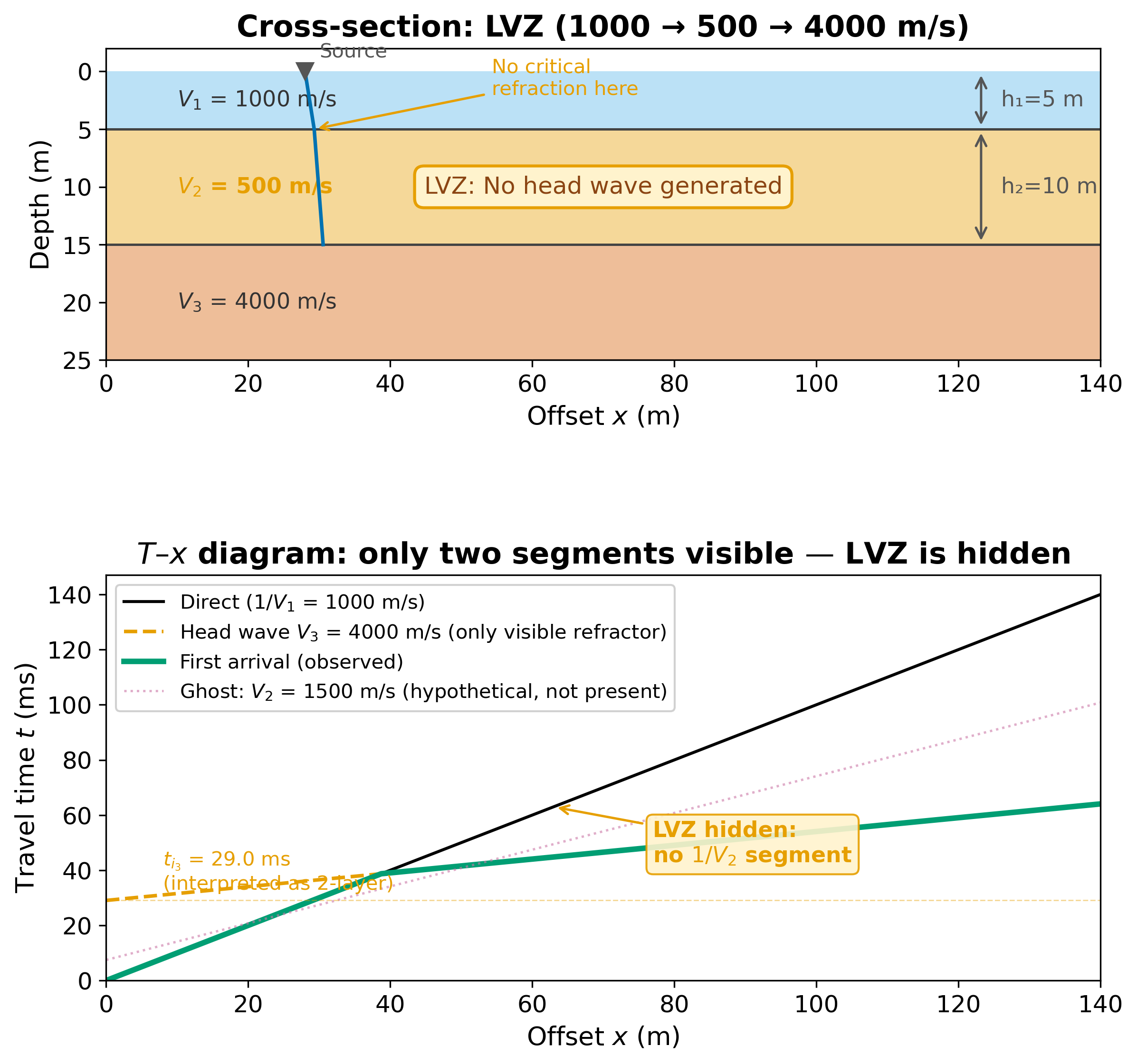
Two-panel figure. Top panel: cross-section with three layers showing V1=1000 m/s over a low-velocity zone V2=500 m/s over V3=4000 m/s; arrows show no critical refraction at the first interface. Bottom panel: travel-time vs. offset plot with only two linear segments (slopes 1/V1 and 1/V3), with annotation showing the LVZ hidden in the record. — Fig. 26 The low-velocity zone problem. When \(V_2 < V_1\), no critical refraction occurs at the first interface, no head wave from the \(V_2\) layer is recorded, and the \(T\)-\(x\) diagram is indistinguishable from a simple two-layer geometry. The interpreted depth to \(V_3\) is greater than the true depth. [Python-generated: `assets/scripts/fig_lvz_traveltime.py`]#

Within the active seismic toolkit, three methods can expose what P-wave first-arrival refraction cannot see.

Seismic reflection is the most direct remedy: reflected waves require only an acoustic impedance contrast (\(Z_2 = \rho_2 V_2 \neq \rho_1 V_1\)), not a velocity increase. A LVZ interface produces a reflection regardless of whether \(V_2 < V_1\) or \(V_2 > V_1\), so seismic reflection surveys directly image boundaries that are invisible to refraction.

Refraction traveltime tomography (SRT) partially mitigates the LVZ problem by inverting the full first-arrival time dataset for a smooth continuous velocity model. Because the tomographic inversion uses all arrivals, it is less susceptible to the blind-zone problem than slope-intercept analysis. However, ray coverage in LVZ regions is inherently sparse, so tomography tends to underestimate the velocity contrast and may not resolve sharp, thin LVZs.

Multichannel Analysis of Surface Waves (MASW) is the most powerful active seismic tool for directly imaging LVZs. Because the phase velocity of surface waves is governed by the shear modulus structure at depth, MASW has no requirement that velocity increase with depth. A velocity inversion that is completely invisible to P-wave first-arrival refraction produces a diagnostic signature in the Rayleigh wave dispersion curve.

S-wave refraction is subject to the same fundamental constraint: it cannot generate a head wave when \(V_{S,2} < V_{S,1}\), so it offers no general solution to the LVZ problem. It is only useful where a P-wave LVZ coincidentally does not coincide with an S-wave LVZ — a specific geological circumstance, not a general fix.

3.2 The Thin Intermediate Layer#

Even when \(V_1 < V_2 < V_3\), the intermediate layer may be too thin to be detected. A head wave from the \(V_2\) interface becomes the first arrival only over a limited crossover distance range. If that window is smaller than the station spacing, the intermediate refractor never appears as a distinct first-arrival segment.

\[x_{c,1} = 2h_1\sqrt{\frac{V_2 + V_1}{V_2 - V_1}}\]

Rule of Thumb

For reliable detection of a layer of velocity \(V_n\) and thickness \(h_n\) beneath a layer of velocity \(V_1\), the station spacing \(\Delta x\) must satisfy approximately \(\Delta x \lesssim h_n \sqrt{(V_n - V_1)/(V_n + V_1)}\). For typical geologic ratios (\(V_n/V_1 \sim 2\)), this implies \(\Delta x \lesssim 0.6 \, h_n\). Layers thinner than the station spacing will not be resolved.

3.3 The Dipping Interface#

When the refractor dips at angle \(\delta\) to the horizontal, a single forward-shot profile produces an apparent velocity that depends on both the true refractor velocity and the dip. To recover the true velocity and dip, a reversed profile is required.

For a down-dip shot (source at the shallow end of the interface):

(63)#\[t_d(x) = \frac{x}{V_1}\sin(\theta_{ic} + \delta) + t_{id}\]

For an up-dip shot (source at the deep end):

(64)#\[t_u(x) = \frac{x}{V_1}\sin(\theta_{ic} - \delta) + t_{iu}\]

Key Equations: Dipping Interface Apparent Velocities

The apparent velocities measured from the \(T\)-\(x\) slopes are:

\[\frac{1}{\alpha_d} = \frac{\sin(\theta_{ic} + \delta)}{V_1}, \qquad \frac{1}{\alpha_u} = \frac{\sin(\theta_{ic} - \delta)}{V_1}\]

The true velocity and dip are recovered from:

\[\delta = \frac{1}{2}\left[\sin^{-1}\!\left(\frac{V_1}{\alpha_d}\right) - \sin^{-1}\!\left(\frac{V_1}{\alpha_u}\right)\right]\]

For small dip angles (\(\delta \lesssim 15\)–\(20°\)):

\[\frac{1}{V_2} \approx \frac{1}{2}\left(\frac{1}{\alpha_d} + \frac{1}{\alpha_u}\right)\]

The reciprocal time (travel time from source \(A\) to the far end equals travel time from source \(B\) to the near end) is a critical quality check: a mismatch indicates a timing error or lateral velocity variation.

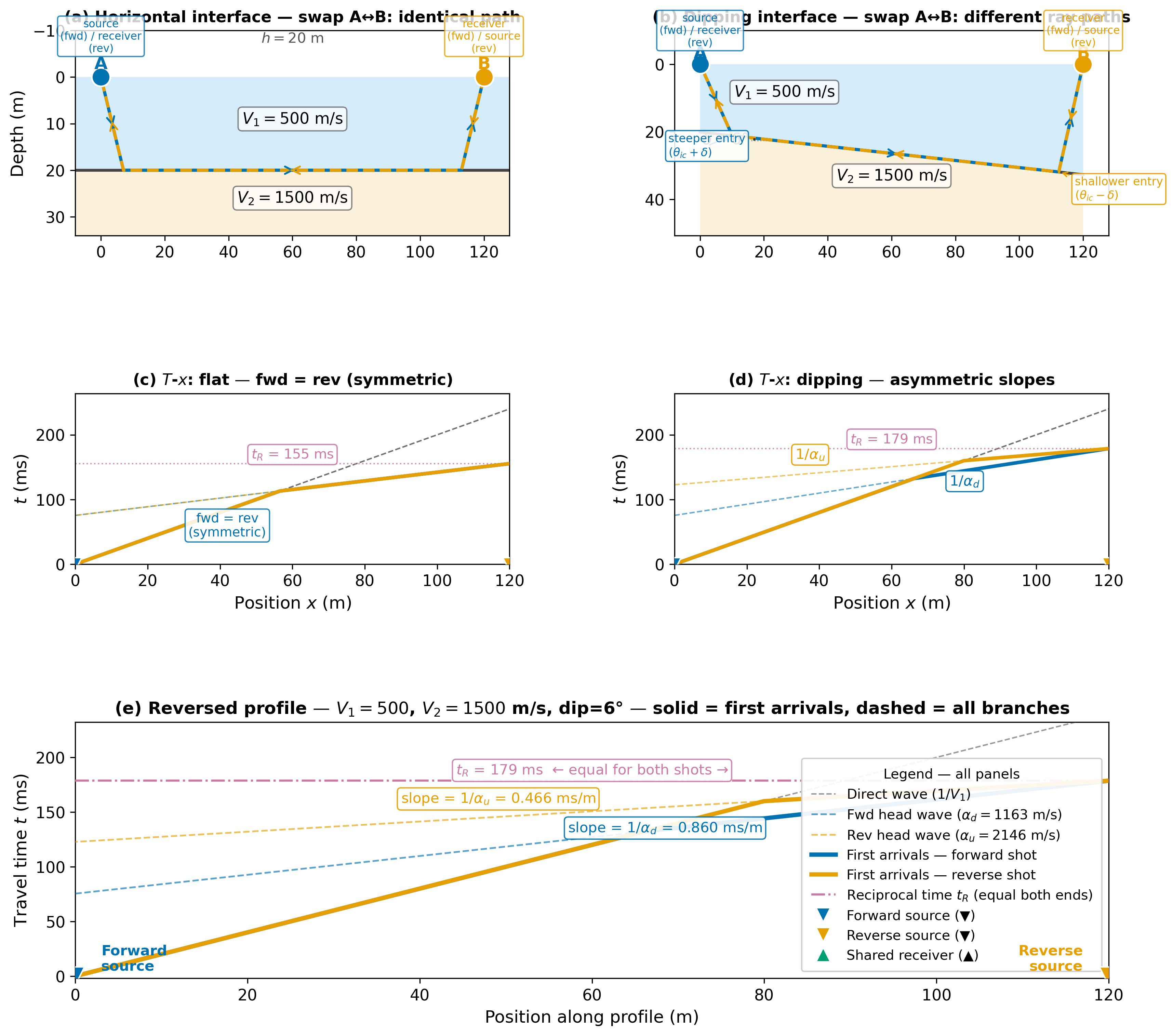
Multi-panel figure comparing horizontal and dipping interface refraction surveys. Cross-sections show ray paths for forward and reverse shots. Travel-time diagrams show parallel head-wave segments for the horizontal case and converging segments with different apparent velocities for the dipping case. The reciprocal time is marked as equal for both shots. — Fig. 27 Reversed refraction profiles over horizontal and dipping interfaces. For a dipping interface, forward and reverse head-wave segments yield different apparent velocities \(\alpha_d\) and \(\alpha_u\) from which the true velocity and dip are recovered. [Python-generated: `assets/scripts/fig_dipping_interface_reversed.py`]#

4. The Forward Problem#

The forward problem for seismic refraction consists of predicting \(T\)-\(x\) curves given a complete specification of layer velocities, thicknesses, and interface orientation. For a horizontally layered model the forward solution is analytic (Eq. (61)).

The complete forward model predicts:

The direct wave arrival: \(t_{dir}(x) = x/V_1\)
The head wave from each interface \(n\): \(t_n(x)\) via Eq. (61)
The crossover distance \(x_{c,n}\) at which head wave \(n\) overtakes the direct wave

\[x_{c} = 2h_1\sqrt{\frac{V_2 + V_1}{V_2 - V_1}}\]

The first-arrival time at any offset is:

\[t_{FA}(x) = \min\!\left[t_{dir}(x),\; t_2(x),\; t_3(x),\; \ldots\right]\]

5. The Inverse Problem#

5.1 Slope-Intercept Inversion#

Given observed first-arrival times as a function of offset, the standard refraction inversion proceeds as follows:

Identify linear segments in the \(T\)-\(x\) diagram and fit them by least squares.
Extract slope = \(1/V_n\) and intercept \(t_{i_n}\) for each segment.
Solve sequentially for layer thicknesses using Eq. (61).
For dipping interfaces, use reversed-profile apparent velocities and Eqs. (63)–(64) to recover true velocity and dip.

Inverse Problem Setup

Data (d): First-arrival travel times \(t_{FA}(x_i)\)
Model (m): Layer velocities \(\{V_n\}\) and thicknesses \(\{h_n\}\) (and dip \(\delta\) for dipping case)
Forward relation: \(d = G(m)\) via Eq. (61)
Key non-uniqueness: LVZs, thin layers, and lateral heterogeneity are all invisible; different Earth models can fit the same \(T\)-\(x\) data within noise
Resolution limit: Layer thicknesses smaller than ~\(0.6\,\Delta x_{station}\) are unresolvable

5.2 The Delay-Time Method for Irregular Refractors#

For surveys where the refractor depth varies smoothly — a common situation over glacially sculpted bedrock or alluvial basins — the delay-time method is more appropriate than slope-intercept inversion.

The delay time \(\delta t_G\) at geophone position \(G\) is:

(65)#\[\delta t_G = \frac{h_G \cos\theta_{ic}}{V_1}\]

The depth to the refractor at \(G\) is recovered from the sum of forward and reverse delay times:

(66)#\[h_G = \frac{V_1 V_2}{2\sqrt{V_2^2 - V_1^2}}\left[\delta t_{F,G} + \delta t_{R,G}\right]\]

This produces a point-by-point refractor profile, graphically equivalent to drawing circular arcs of radius \(h_G\) beneath each geophone and finding their common tangent envelope.

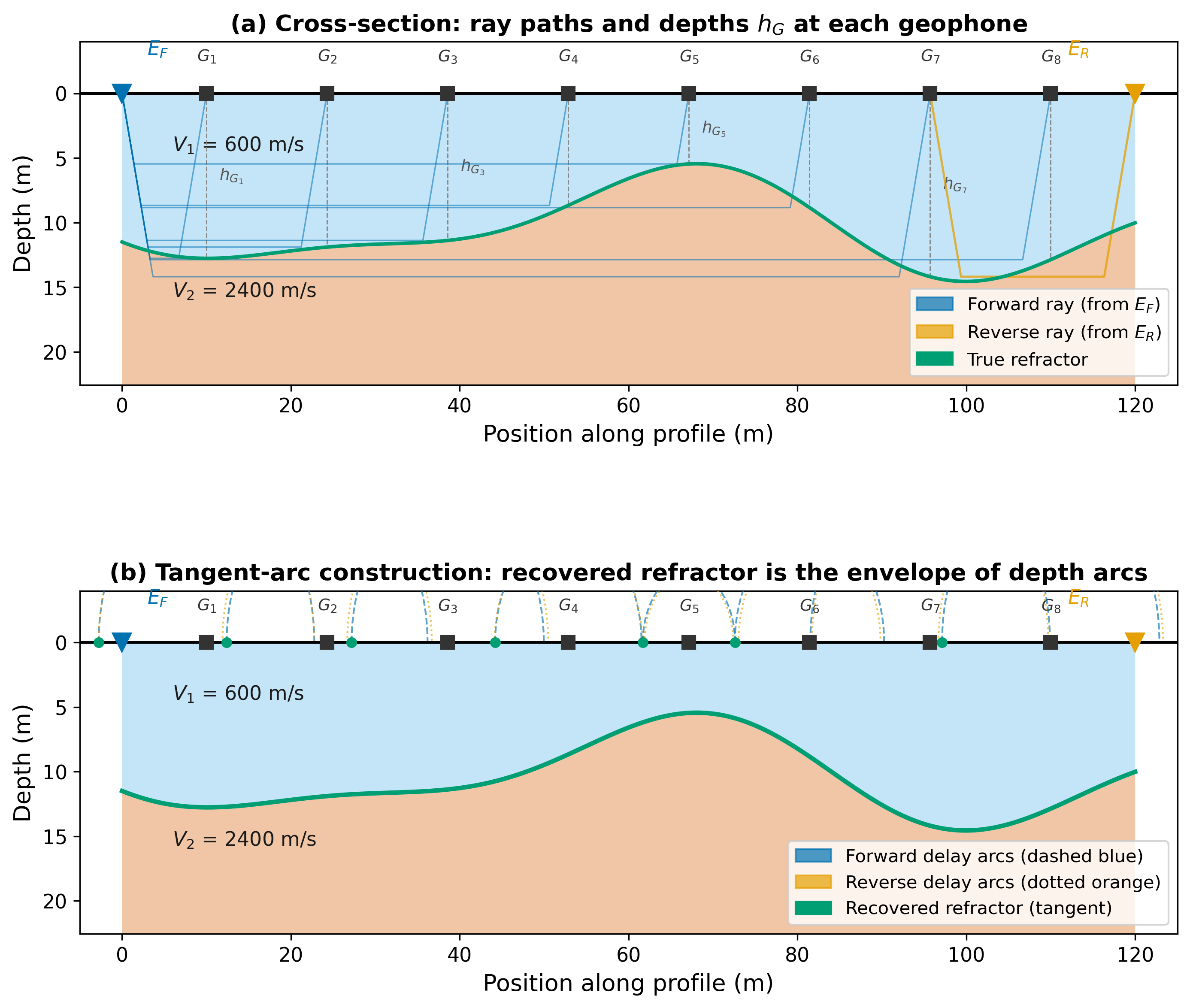
Two-panel figure. Top panel: cross-section with undulating refractor between V1 and V2 layers, showing forward and reverse ray paths to eight geophone positions. Bottom panel: tangent-arc construction showing circular arcs of radius h_G beneath each geophone; the refractor surface is the common tangent envelope to all arcs. — Fig. 28 The delay-time method for mapping an irregular refractor. The depth \(h_G\) at each geophone is computed from Eq. (66) using forward and reverse delay times. The refractor surface is the common tangent to all arcs. [Python-generated: `assets/scripts/fig_delay_time_method.py`]#

6. Worked Example: Puget Lowland Site Investigation#

Consider a shallow refraction survey conducted across a Quaternary terrace in the Puget Lowland — a common scenario for dam-foundation investigations, liquefaction hazard assessment, or buried channel mapping in the Seattle metropolitan area. The site is interpreted to have three layers:

Layer	Description	True velocity
1	Loose fill and organic soil	\(V_1 = 350\) m/s
2	Dense glacial outwash gravel	\(V_2 = 1{,}650\) m/s
3	Competent sandstone (Renton Fm.)	\(V_3 = 4{,}200\) m/s

A 72-m geophone spread records a forward shot. The following slopes and intercepts are read from the \(T\)-\(x\) diagram:

Segment	Slope (ms/m)	Velocity (m/s)	Intercept \(t_i\) (ms)
Direct	2.857	350	0
Head wave \(V_2\)	0.606	1650	6.1
Head wave \(V_3\)	0.238	4200	19.4

Step 1: Compute \(h_1\) from the \(V_2\) intercept time:

\[\theta_{ic,12} = \sin^{-1}\!\left(\frac{350}{1650}\right) = 12.3°, \qquad h_1 = \frac{t_{i_2} V_1}{2\cos\theta_{ic,12}} = \frac{0.0061 \times 350}{2 \times 0.9770} = 1.09 \text{ m}\]

Step 2: Compute \(h_2\) from the \(V_3\) intercept time using Eq. (62):

\[h_2 \approx 14.6 \text{ m}\]

The bedrock surface lies approximately 15.7 m below the surface (\(h_1 + h_2\)).

Concept Check

Q1. If the outwash gravel layer (\(V_2 = 1650\) m/s) were replaced by clay with \(V_2 = 300\) m/s, how would the \(T\)-\(x\) diagram appear, and how would the interpreted depth to bedrock compare with the true depth?

Q2. The hammer-source timing has an uncertainty of \(\pm 1\) ms. Propagate this timing uncertainty through the \(h_1\) calculation. Is the depth uncertainty acceptable for a dam-foundation application?

Q3. A reversed shot yields a \(V_3\)-segment slope of 0.255 ms/m (apparent velocity 3921 m/s). Using the small-dip approximation, estimate the dip angle of the sandstone surface.

7. Uncertainty in Refraction Interpretation#

Picking uncertainty. First-arrival picking errors of 0.5–2 ms are common. A 1 ms error in the intercept time propagates to a depth error \(\delta h = V_1 \delta t / (2\cos\theta_{ic})\).

Velocity gradient effects. A gradient in the shallowest layer causes the \(T\)-\(x\) direct-wave segment to curve upward, systematically biasing intercept-time estimates.

Lateral heterogeneity. A lateral velocity gradient (buried channel, fault) modifies the apparent velocity of head-wave segments, producing an artifact indistinguishable from dip in a single-profile survey.

Non-uniqueness. Different combinations of layer velocities, thicknesses, and dip angles can produce \(T\)-\(x\) curves that are indistinguishable within noise. Integration with borehole and other geophysical data is essential.

Source	Effect	Magnitude
First-arrival picking error (\(\pm\)1 ms)	Depth error \(\delta h = V_1 \delta t / 2\cos\theta_{ic}\)	0.1–5 m
Velocity gradient in top layer	Curved direct-wave segment; biased intercepts	Depends on gradient
Lateral velocity variation	Apparent dip artifact; false structure	Can be large
LVZ (undetected)	Systematic underestimate of depth to refractor	Proportional to LVZ thickness
Station spacing too large	Missing intermediate layer	\(\delta h \sim \Delta x / 0.6\)

8. Research Horizon#

Near-surface velocity imaging has undergone a methodological revolution driven by dense ambient-noise recordings and machine-learning phase pickers.

Current Research Highlights (2022–2025)

Full-waveform inversion (FWI) of shallow seismic data: Rather than picking only first arrivals, FWI minimizes the waveform misfit across the entire shot gather, recovering smooth velocity models that resolve both first-order interfaces and gradual transitions. This substantially relaxes the blind-zone limitation inherent to head-wave methods.

Distributed Acoustic Sensing (DAS) refraction surveys: Fiber-optic cables buried in urban environments record ambient seismic noise and active-source shots with centimetre-scale spatial sampling, enabling refraction imaging at unprecedented resolution — directly relevant to PNSN and EarthScope urban seismology efforts in Seattle.

Machine-learning first-arrival pickers: Phase-picking models (e.g., PhaseNet, EQTransformer) trained on earthquake waveforms transfer surprisingly well to shallow active-source gathers, reducing picking time from hours to seconds and providing automated uncertainty estimates (Zhu et al., 2019, Seismological Research Letters).

For students interested in graduate research: EarthScope SSBW workshops, the SCOPED open notebooks project (scoped.codes), and IRIS/EarthScope education resources are good entry points.

9. Societal Relevance#

Shallow seismic refraction is among the most widely deployed geophysical methods in geotechnical practice. In the Pacific Northwest, the technique is applied routinely to:

Why It Matters Beyond the Classroom

Liquefaction hazard assessment: Mapping the depth to the water table and to competent bearing materials beneath Seattle neighborhoods built on Holocene deltaic and glaciolacustrine deposits informs building codes and emergency planning for Cascadia megathrust scenarios.

Debris flow and landslide investigations: Mapping the bedrock-colluvium interface on the steep volcanic slopes of Mount Rainier and the Cascades, where this interface controls pore-pressure accumulation and slope failure initiation.

Transportation infrastructure: WSDOT and Sound Transit use refraction surveys to characterize the Renton Formation and Vashon Drift for tunnel and light-rail alignment in the Seattle basin.

For further exploration: USGS Open-File Report 88-296 (Haeni 1988, public domain) provides a detailed field guide; EarthScope/IRIS Teachable Moments include shallow-structure case studies.

AI Literacy: AI as a Reasoning Partner in Inverse Problems#

AI Prompt Lab — Checking Your Refraction Inversion

Prompt 1 (Derivation check): “I am solving for layer thickness in a three-layer seismic refraction problem. My travel-time equation for the second head wave is \(t_3 = x/V_3 + 2h_1\sqrt{V_3^2 - V_1^2}/(V_3 V_1) + 2h_2\sqrt{V_3^2 - V_2^2}/(V_3 V_2)\). Please derive the expression for \(h_2\) in terms of the intercept time \(t_{i_3}\), the already-known thickness \(h_1\), and the layer velocities.”

Evaluate the AI response for dimensional consistency and correct isolation of \(h_2\). Verify by substituting back into the travel-time equation.

Prompt 2 (Failure mode recognition): “In a seismic refraction survey, the \(T\)-\(x\) diagram shows only two straight-line segments even though a borehole nearby shows three distinct velocity units. What geological and interpretive explanations should a geophysicist consider?”

Evaluate: Does the AI distinguish between the LVZ problem and the thin-layer problem? Does it recommend specific additional data collection strategies?

Evaluation criterion: A reliable AI response will state the assumptions explicitly (horizontal layers, no lateral variation, monotonically increasing velocity) and flag when those assumptions may be violated.

10. Course Connections#

Prior lectures: The critical angle derivation (Lecture 5) and the single-layer \(T\)-\(x\) equations (Lecture 6) are the direct precursors.
Next lecture: Lecture 8 (Seismic Reflection I) treats the same layered-Earth geometry but focuses on the reflection branch — the wavefront that turns back at the interface rather than continuing along it.
Lab 3: Students pick first arrivals from a real field shot gather from the Puget Lowland area, fit multi-layer models, and quantify depth uncertainty.
Lecture 13 (Seismic Tomography): The delay-time concept introduced here is a pedagogical precursor to tomographic ray-path integrals.
Cross-method connection: The velocity contrasts that drive refraction head waves also control electrical resistivity contrasts, acoustic impedance for reflection surveys, and density anomalies detectable by gravity.


Course LOs addressed	LO-1, LO-2, LO-3, LO-4, LO-5, LO-6
Learning outcomes practiced	LO-OUT-A, LO-OUT-B, LO-OUT-C, LO-OUT-D, LO-OUT-E
Prior lecture	Lecture 6 — Seismic Refraction I (horizontal single-layer model, critical angle, \(T\)-\(x\) straight-line interpretation)
Next lecture	Lecture 8 — Introduction to Seismic Reflection
Lab connection	Lab 3: Refraction — students fit multi-layer models to real field shot gathers