Wavefronts, Rays, and Snell’s Law

Wavefronts, Rays, and Snell’s Law#

1. The Geoscientific Question#

A seismologist at the Pacific Northwest Seismic Network notices something surprising. An earthquake occurs 50 km offshore of Westport, Washington, at a depth of 30 km in the subducting Juan de Fuca plate. The P-wave recorded at a station in Olympia arrives from an unexpected direction — not along the straight line from the source, but from a steeper angle. The wave has been bent by the velocity structure of the crust and upper mantle.

This bending is not random. It follows a precise law — Snell’s law — that governs ray geometry wherever velocity changes. The same law applies to light refracting through a prism, sound waves bending in the ocean, and seismic waves curving through the Earth. To use seismic waves as probes of Earth structure, one must understand how their paths respond to velocity contrasts. This lecture develops that understanding from two complementary perspectives: the wave picture (Huygens’ principle) and the variational principle (Fermat’s principle). Both yield the same result — Snell’s law — but each provides different physical insight.

The Central Question

When a seismic wave encounters a velocity contrast, its path bends. What law governs this bending, and how is it derived from the physics of wave propagation?

2. Governing Physics: Wavefronts and Rays#

2.1 Wavefronts and Rays in Homogeneous Media#

A wavefront is a surface of constant phase — the locus of all points reached by the wave at the same instant. In a homogeneous, isotropic medium, wavefronts from a point source are spherical (3D) or circular (2D), expanding outward at speed \(V\).

A ray is the direction of energy propagation. In an isotropic medium, rays are always perpendicular to wavefronts. A ray from a point source is a straight line radiating outward — rays are the normals to the expanding spheres.

At distances much larger than the wavelength, the wavefront appears locally flat — a plane wave. The plane-wave approximation is the foundation of ray theory and is valid whenever structures of interest are much larger than the dominant wavelength.

2.2 Wavefronts and Rays in Heterogeneous Media#

When the wave speed varies spatially — \(V = V(\mathbf{x})\) — wavefronts deform. The part of the wavefront in faster material advances farther in a given time interval; the part in slower material lags behind. The result: wavefronts are no longer spherical, and rays are no longer straight.

Two-panel figure. Panel (a) shows a point source at the surface with semicircular wavefronts expanding downward in a uniform blue medium, with straight downward-pointing ray arrows perpendicular to each wavefront. Panel (b) shows the same source above a medium containing a low-velocity elliptical anomaly (sedimentary basin or magma chamber) outlined by a dashed red ellipse. The velocity field is shown as a colour mesh. Rays bend into the slow anomaly, and wavefronts retard (bulge inward) inside it. 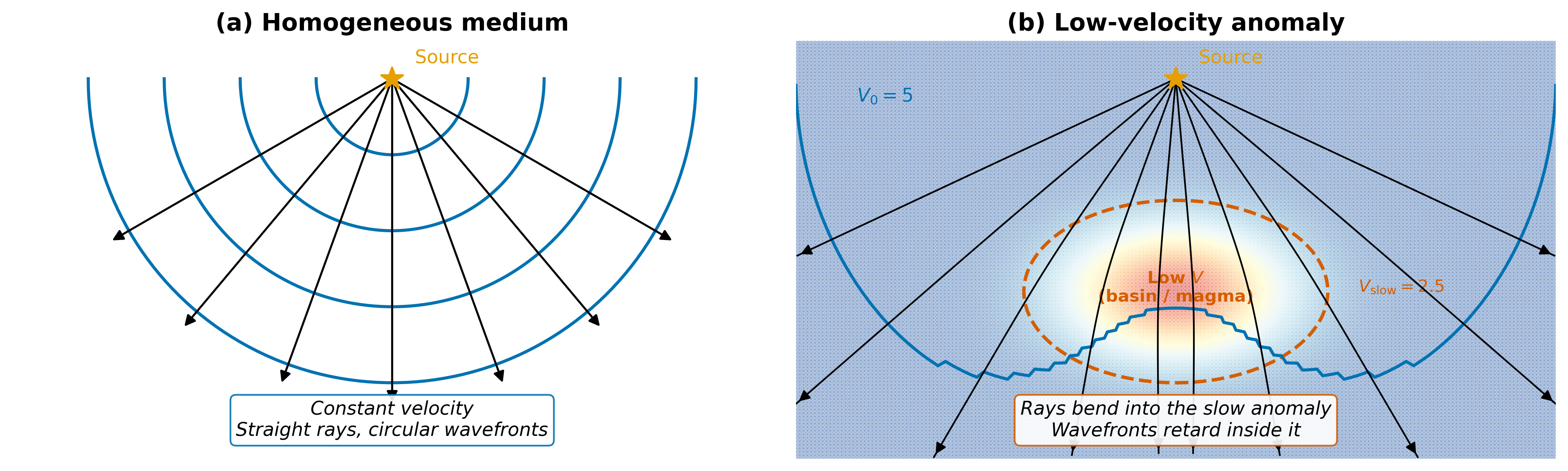— Fig. 14 **Figure 5.1.** Wavefronts and rays in (a) a homogeneous isotropic medium: circular wavefronts, straight rays, and (b) a medium with a low-velocity anomaly (basin / magma chamber): rays bend into the slow region and wavefronts retard inside it. Rays always point perpendicular to wavefronts in isotropic media. [Python-generated. Script: `assets/scripts/fig_wavefronts_isotropic_hetero.py`]#

Key Concept: Rays Bend Toward Slow Regions

In a medium where velocity increases to the right, the right side of the wavefront advances faster, tilting the wavefront and curving the ray to the left — toward the slower region. Rays always bend toward lower-velocity material. This is the qualitative content of Snell’s law: the angle from the normal is smaller in the slower medium.

3. Mathematical Framework#

3.1 Notation#

Notation

Symbol	Quantity	Units	Type
\(\theta_1\)	Angle of incidence (from interface normal)	rad or °	scalar
\(\theta_2\)	Angle of refraction (from interface normal)	rad or °	scalar
\(V_1\), \(V_2\)	Wave speed in medium 1, medium 2	m/s	scalars
\(p\)	Ray parameter \(= \sin\theta / V\)	s/m	scalar
\(T\)	Travel time	s	scalar
\(d\)	Horizontal offset between source and receiver	m	scalar
\(h\)	Layer thickness	m	scalar
\(x\)	Horizontal position of the refraction point	m	scalar
\(ds\)	Infinitesimal arc length along a ray	m	scalar

3.2 Huygens’ Principle#

Huygens’ principle (1678) states: every point on a wavefront acts as a secondary point source, emitting a spherical wavelet. The new wavefront at time \(t + \Delta t\) is the envelope — the surface tangent to all secondary wavelets.

This is not merely a geometric trick. It is a consequence of the Kirchhoff integral representation of the wave equation: the wavefield at any point can be expressed as a superposition of contributions from all points on a prior wavefront, each radiating as a Green’s function.

Diagram showing a curved wavefront at time t-zero on the left. Five evenly spaced points on this wavefront are marked as secondary sources, each emitting a circular wavelet of radius V times delta-t. A new wavefront at time t-zero plus delta-t is drawn as the envelope tangent to all five wavelets on the right side. Arrows between the two wavefronts show the propagation direction, perpendicular to the wavefronts. Labels identify the initial wavefront, point sources, secondary wavelets, and the new wavefront. 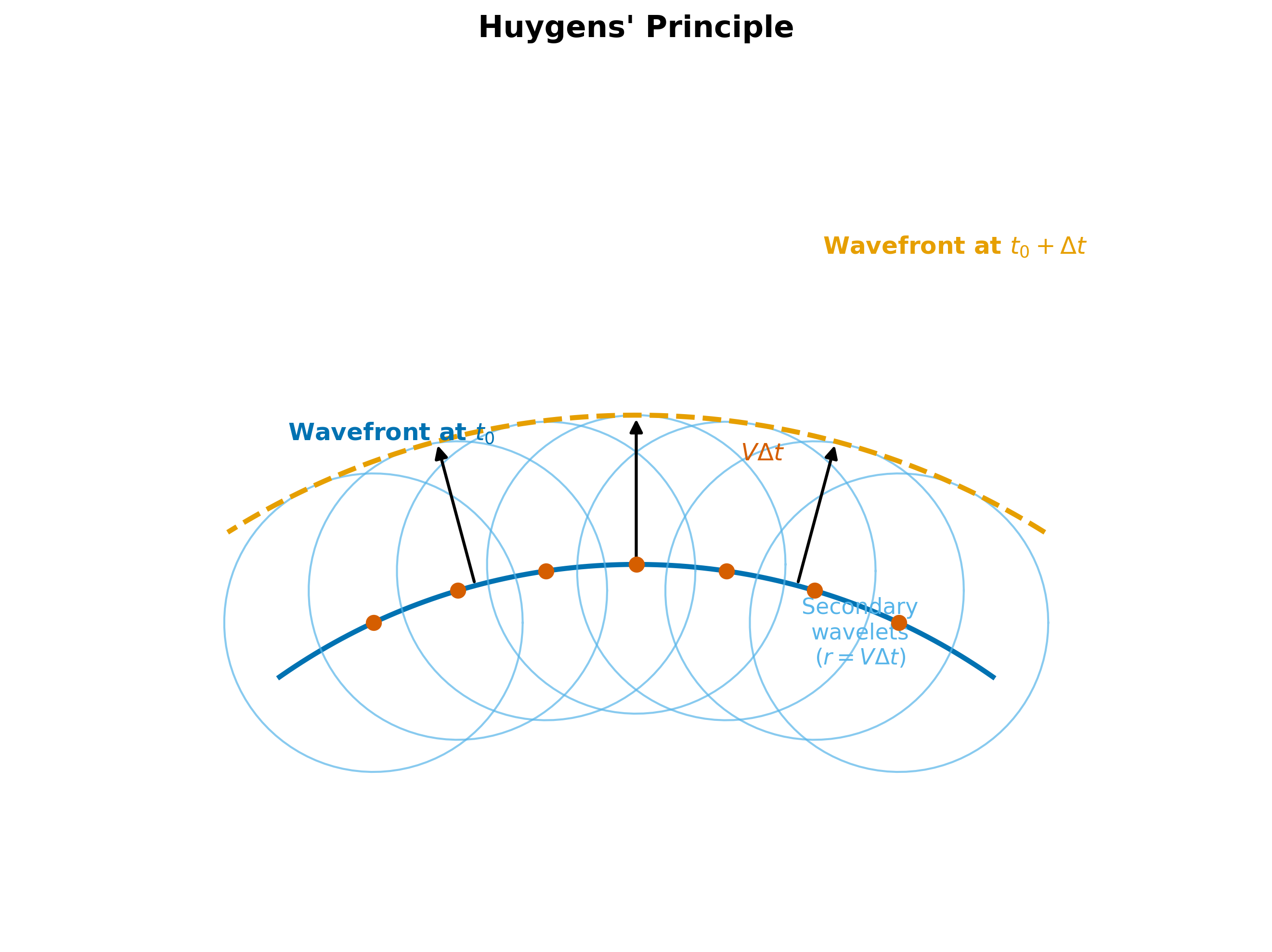— Fig. 15 **Figure 5.2.** Huygens’ principle: each point on a wavefront radiates a secondary spherical wavelet. The new wavefront is the envelope of all wavelets. In a homogeneous medium, the result is a wavefront that has advanced uniformly. [Python-generated. Script: `assets/scripts/fig_huygens_principle.py`]#

3.3 Deriving Snell’s Law from Huygens’ Construction#

Consider a plane wavefront impinging on a flat interface between medium 1 (speed \(V_1\)) and medium 2 (speed \(V_2 > V_1\)). The wavefront first strikes the interface at point \(A\) at time \(t = 0\). A second point on the wavefront, at point \(C\), is still in medium 1 and must travel a distance \(BC = V_1\,\Delta t\) to reach the interface at point \(B\).

During the same interval \(\Delta t\), the Huygens wavelet from \(A\) has expanded into medium 2 with radius \(AE = V_2\,\Delta t\). The refracted wavefront is the tangent line from \(B\) to this wavelet.

From the geometry of the two right triangles sharing the hypotenuse \(AB\):

(38)#\[ \sin\theta_1 = \frac{BC}{AB} = \frac{V_1\,\Delta t}{AB} \]

(39)#\[ \sin\theta_2 = \frac{AE}{AB} = \frac{V_2\,\Delta t}{AB} \]

Dividing (38) by (39), the shared quantities \(\Delta t\) and \(AB\) cancel:

(40)#\[ \frac{\sin\theta_1}{\sin\theta_2} = \frac{V_1}{V_2} \]

Rearranged into the canonical form:

(41)#\[ \frac{\sin\theta_1}{V_1} = \frac{\sin\theta_2}{V_2} = p \]

Key Equation: Snell’s Law

\[ \frac{\sin\theta_1}{V_1} = \frac{\sin\theta_2}{V_2} = p \]

The quantity \(p\) is the ray parameter — it is constant along the entire ray path through any number of horizontal layers. Physically, \(p\) is the horizontal component of the slowness vector \(\mathbf{s} = \hat{n}/V\), where \(\hat{n}\) is the ray direction.

Units: \([\sin\theta]/[V] = \text{dimensionless}/(\text{m/s}) = \text{s/m}\) ✓

Consequences:

\(V_2 > V_1\): ray bends away from normal (\(\theta_2 > \theta_1\)) — into the faster medium
\(V_2 < V_1\): ray bends toward normal (\(\theta_2 < \theta_1\)) — into the slower medium
Vertical incidence (\(\theta_1 = 0\)): no bending regardless of velocity contrast

Geometric construction for Snell's law derivation. A horizontal interface separates medium 1 above with velocity V_1 in blue from medium 2 below with velocity V_2 in green. An incident wavefront arrives from the upper left at angle theta_1 from the normal. Point A on the interface emits a Huygens wavelet into medium 2 with radius V_2 times delta-t. Point C on the wavefront travels a distance V_1 times delta-t to reach the interface at B. Two right triangles share the hypotenuse AB, with the sine relations labeled. The refracted wavefront extends from B tangent to the wavelet, at angle theta_2 from the normal. 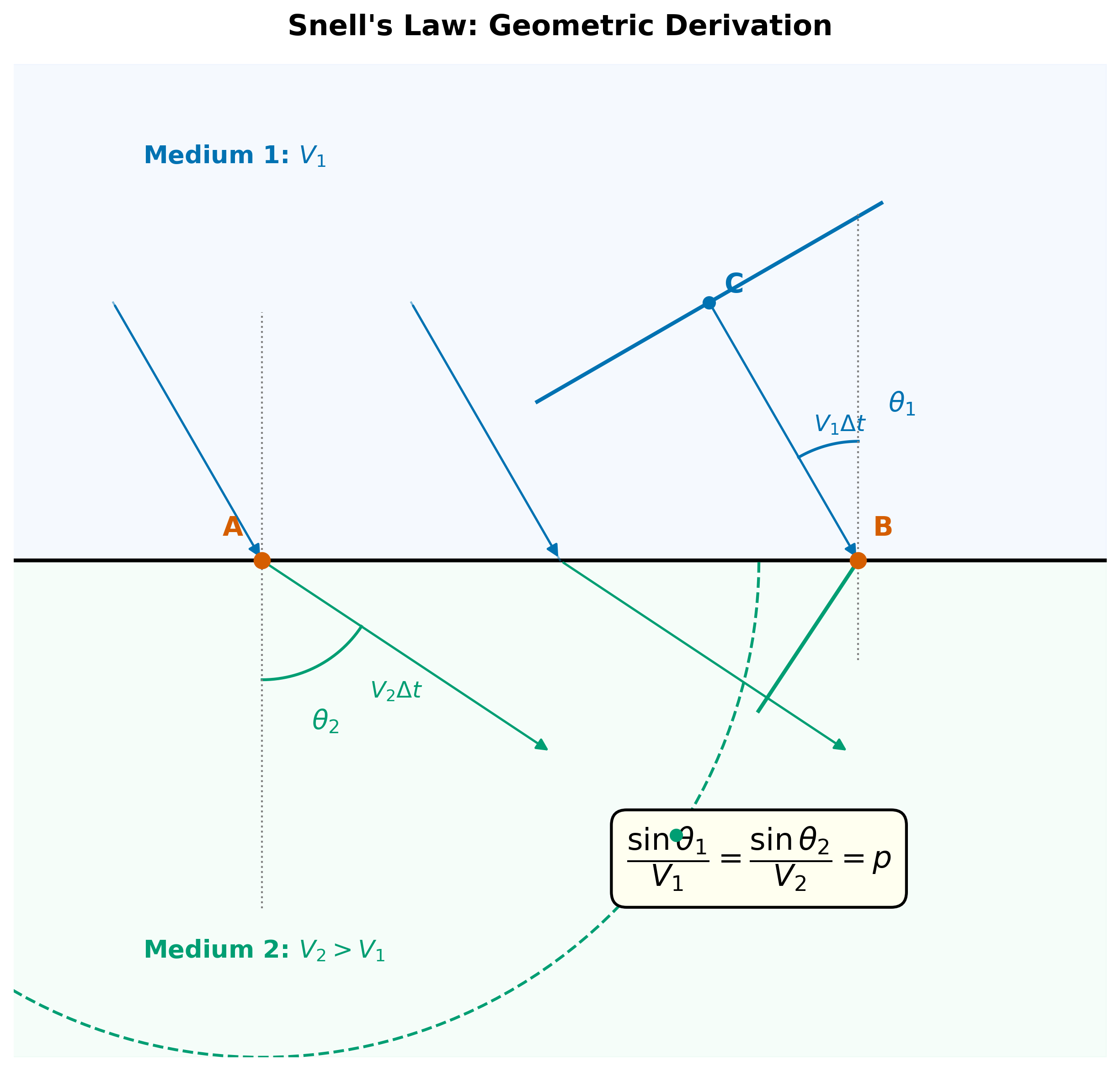— Fig. 16 **Figure 5.3.** Geometric derivation of Snell’s law from Huygens’ construction. Two right triangles sharing the hypotenuse \(AB\) yield \(\sin\theta_1/V_1 = \sin\theta_2/V_2\). [Python-generated. Script: `assets/scripts/fig_snell_law_geometry.py`]#

3.4 The Ray Parameter as a Conserved Quantity#

The ray parameter \(p\) is invariant along a ray passing through any number of horizontal layers:

(42)#\[ p = \frac{\sin\theta_1}{V_1} = \frac{\sin\theta_2}{V_2} = \frac{\sin\theta_3}{V_3} = \cdots \]

This conservation law is analogous to the conservation of horizontal momentum in classical mechanics. In a medium with horizontal symmetry (properties vary only with depth), the horizontal component of the slowness vector is conserved — a direct consequence of translational invariance along the interface.

For a continuously varying velocity \(V(z)\), the ray parameter is still conserved:

(43)#\[ p = \frac{\sin\theta(z)}{V(z)} = \text{constant along the ray} \]

A ray launched at angle \(\theta_0\) from the surface with surface velocity \(V_0\) has \(p = \sin\theta_0/V_0\). As the ray descends into faster material, \(V\) increases, so \(\sin\theta\) must increase to keep \(p\) constant — the ray tilts more and more toward horizontal. When \(\sin\theta = 1\) (ray is horizontal), the ray has reached its turning depth, where \(V(z_\text{turn}) = 1/p\), and it begins curving back upward.

3.5 Fermat’s Principle and Snell’s Law#

Snell’s law can be derived independently from a variational principle — Fermat’s principle of least time (more precisely, stationary time): the actual ray path between two points is the one for which the travel time is stationary with respect to small perturbations of the path.

Consider a source at point \(A\) in medium 1 at height \(h\) above the interface, and a receiver at point \(B\) in medium 2 at depth \(h\) below the interface, horizontally separated by distance \(d\). The ray crosses the interface at a horizontal position \(x\) from \(A\).

Geometric diagram showing a source A at height h above a horizontal interface and a receiver B at depth h below the interface, horizontally separated by distance d. A ray path from A crosses the interface at point O at horizontal distance x from A, then continues to B at horizontal distance d minus x. The angle of incidence theta_i at the crossing point is measured from the interface normal. Three alternative paths are shown as dashed gray lines with longer travel times, while the solid blue path shows the minimum-time trajectory satisfying Snell's law. A red box shows the travel time formula T equals the square root of h-squared plus x-squared divided by V_1 plus the square root of h-squared plus d-minus-x squared divided by V_2. 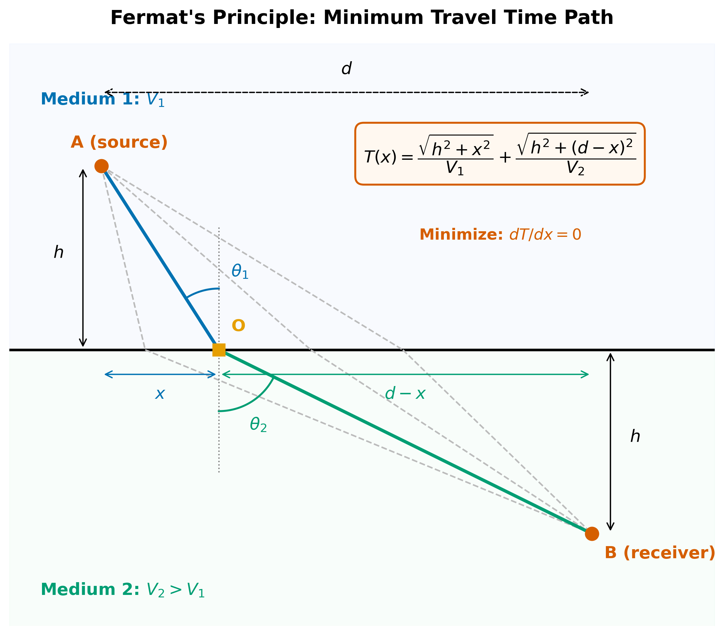— Fig. 17 **Figure 5.4.** Fermat’s principle geometry. The travel time \(T(x)\) depends on where the ray crosses the interface. The minimum-time path satisfies Snell’s law. [Python-generated. Script: `assets/scripts/fig_fermat_principle.py`]#

The total travel time as a function of the crossing position \(x\):

(44)#\[ T(x) = \frac{\sqrt{h^2 + x^2}}{V_1} + \frac{\sqrt{h^2 + (d-x)^2}}{V_2} \]

To find the path of minimum time, set \(dT/dx = 0\):

(45)#\[ \frac{dT}{dx} = \frac{x}{V_1\sqrt{h^2 + x^2}} - \frac{(d-x)}{V_2\sqrt{h^2 + (d-x)^2}} = 0 \]

Recognizing from the geometry that:

(46)#\[ \sin\theta_1 = \frac{x}{\sqrt{h^2 + x^2}}, \qquad \sin\theta_2 = \frac{d-x}{\sqrt{h^2 + (d-x)^2}} \]

the condition \(dT/dx = 0\) becomes:

(47)#\[ \frac{\sin\theta_1}{V_1} = \frac{\sin\theta_2}{V_2} \]

This is Snell’s law, derived purely from the requirement that the ray path minimizes travel time.

Key Concept: Two Derivations, One Law

Snell’s law can be derived from:

Huygens’ construction — a geometric argument using wavefront geometry at the interface
Fermat’s principle — a variational argument requiring stationary travel time

The Huygens derivation provides geometric intuition. The Fermat derivation is more powerful: it generalizes to curved interfaces, continuously varying media, and non-planar wavefronts. In all cases, the ray parameter \(p = \sin\theta/V\) is conserved — a consequence of the medium’s horizontal translational symmetry.

Units check: \([dT/dx] = \text{s/m}\). Each term: \([\text{m}/((\text{m/s})\cdot\text{m})] = \text{s/m}\) ✓

3.6 Rays in a Continuously Varying Medium#

In the real Earth, velocity generally increases with depth due to increasing pressure. For a medium with \(V(z)\) increasing downward, the ray parameter conservation \(p = \sin\theta(z)/V(z)\) causes rays launched at non-vertical angles to curve continuously — arcing downward, then turning back upward when \(V(z) = 1/p\), and returning to the surface.

The geometry produces a characteristic pattern: steeper rays (smaller \(p\)) penetrate deeper and return at greater horizontal distances. This relationship between ray parameter and epicentral distance is the basis for interpreting travel-time curves from distant earthquakes.

Cross-section showing the Earth's surface at the top and depth increasing downward. A source at the surface emits five rays at different takeoff angles. The velocity increases linearly with depth, shown as a color gradient from light blue at the surface to dark blue at depth. Each ray curves smoothly downward and then back up, with steeper rays penetrating deeper and emerging at greater distances. Dashed horizontal lines mark the turning depth for each ray, labeled with the velocity at that depth. The ray parameter p is labeled for each ray. 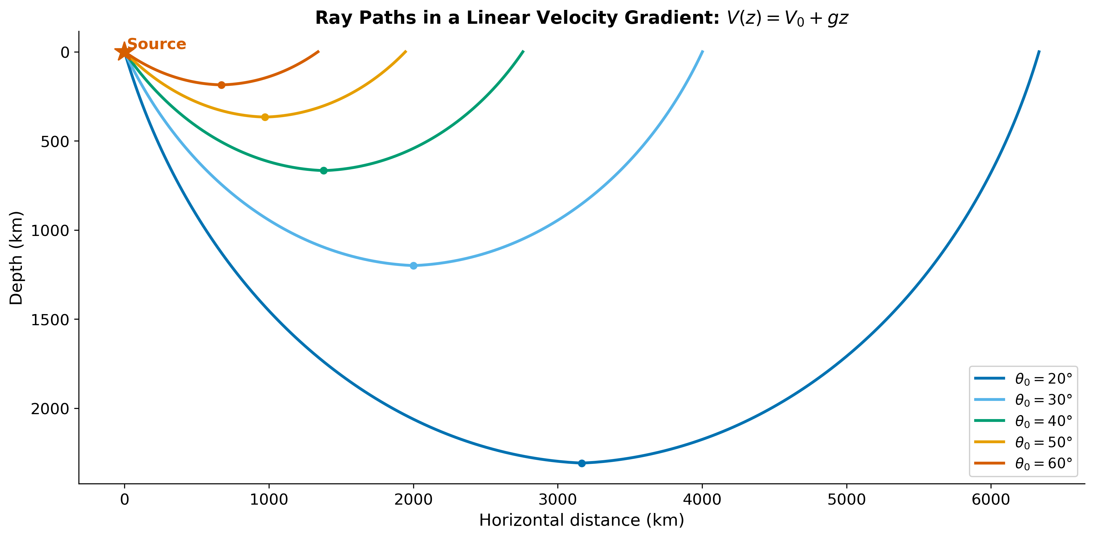— Fig. 18 **Figure 5.5.** Ray paths in a medium with velocity increasing linearly with depth. Steeper rays (smaller \(p\)) penetrate deeper and emerge at greater epicentral distances. Each ray turns at the depth where \(V(z) = 1/p\). [Python-generated. Script: `assets/scripts/fig_ray_bending_gradient.py`]#

3.7 Reflection at an Interface#

So far we have focused on the refracted (transmitted) ray. But at every velocity contrast, a wave also reflects. The reflected ray remains in medium 1, and its angle obeys Snell’s law with the same velocity on both sides:

(48)#\[ \frac{\sin\theta_i}{V_1} = \frac{\sin\theta_r}{V_1} \quad\Longrightarrow\quad \theta_r = \theta_i \]

The angle of reflection equals the angle of incidence — both measured from the interface normal. This is the law of reflection, and it is simply Snell’s law applied within a single medium.

Key Concept

At any velocity contrast, a seismic wave simultaneously reflects and refracts. The relative amplitudes depend on the impedance contrast (§3.9). Only when the media on both sides are identical does the reflected wave vanish entirely.

3.8 Mode Conversion: P–SV Coupling at Interfaces#

When a P-wave strikes an interface at oblique incidence, the boundary conditions — continuity of displacement and traction across the interface — require the generation of both P- and S-waves on each side. A single incident P-wave produces up to four outgoing waves:

Reflected P — angle \(\theta_{P1}^r\) in medium 1
Reflected SV — angle \(\theta_{S1}^r\) in medium 1
Transmitted P — angle \(\theta_{P2}^t\) in medium 2
Transmitted SV — angle \(\theta_{S2}^t\) in medium 2

All four angles are governed by the generalized Snell’s law — a single ray parameter \(p\) for the entire wavefield at the interface:

(49)#\[ p = \frac{\sin\theta_{P1}}{V_{P1}} = \frac{\sin\theta_{S1}}{V_{S1}} = \frac{\sin\theta_{P2}}{V_{P2}} = \frac{\sin\theta_{S2}}{V_{S2}} \]

Since \(V_S < V_P\) in any given medium, the converted S-wave always propagates at a steeper angle (closer to the normal) than the corresponding P-wave. The same logic applies to an incident SV-wave — it generates reflected and transmitted P and SV.

Diagram of P-SV mode conversion at a planar interface. An incident P-wave arrives from the upper left at angle theta_P1 from the normal. At the interface, four outgoing rays emerge — reflected P and reflected SV going to the upper right in medium 1, and transmitted P and transmitted SV going to the lower right in medium 2. The reflected SV is steeper than the reflected P because V_S1 is less than V_P1. The transmitted P is wider than the transmitted SV. All four angles are governed by a single ray parameter p, shown in the generalized Snell's law equation at the bottom. Small double arrows on each ray indicate particle motion direction — along the ray for P-waves, perpendicular to the ray for SV-waves. 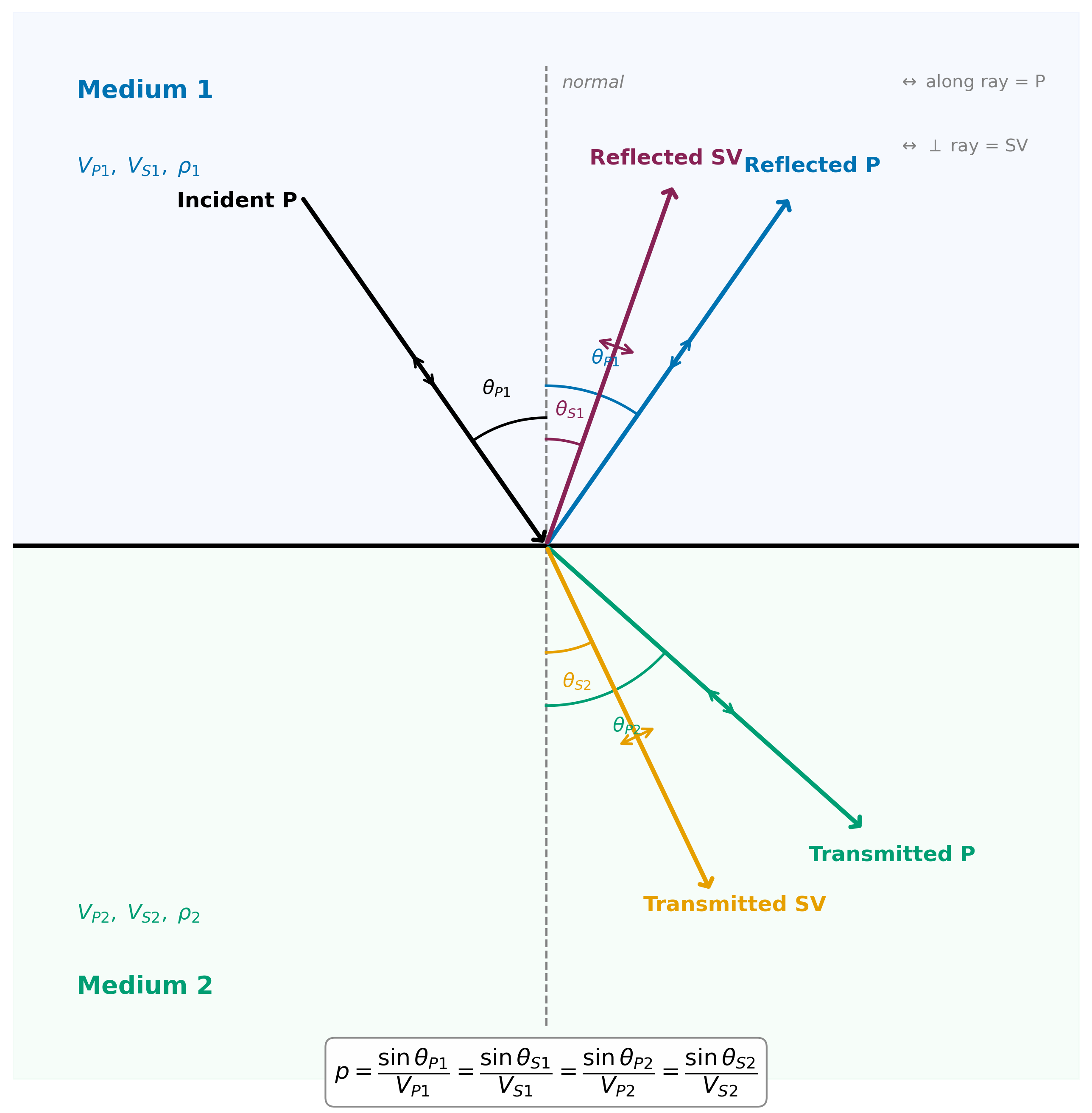— Fig. 19 **Figure 5.6.** P–SV mode conversion at a planar interface. A single incident P-wave generates four outgoing waves. All angles are related by the generalized Snell’s law with a single ray parameter \(p\). The S-waves are always steeper (closer to the normal) than the P-waves because \(V_S < V_P\). Small arrows indicate particle-motion direction: longitudinal (along ray) for P, transverse (perpendicular) for SV. [Python-generated. Script: `assets/scripts/fig_psv_mode_conversion.py`]#

SH Waves Do Not Convert

SH motion (horizontal, parallel to the interface) is decoupled from P–SV motion in isotropic media. An incident SH wave generates only reflected and transmitted SH — no P or SV conversion. Conversely, an incident P or SV wave generates no SH.

3.9 Amplitude at an Interface: Reflection and Transmission Coefficients#

Snell’s law (and its generalized form) dictate the angles of reflected and transmitted waves. The amplitudes are determined by the boundary conditions: continuity of displacement and stress across the interface. The key material property controlling how much energy reflects is the acoustic impedance:

(50)#\[ Z = \rho\, V \]

where \(\rho\) is density and \(V\) is wave speed. Units: \(\mathrm{kg/(m^2 \cdot s)}\), also called rayls.

Normal-incidence coefficients. For a wave arriving perpendicular to the interface (\(\theta = 0\)), the displacement amplitude ratios simplify to:

(51)#\[ R = \frac{Z_2 - Z_1}{Z_2 + Z_1}, \qquad T = \frac{2\,Z_1}{Z_2 + Z_1} \]

where \(Z_1 = \rho_1 V_1\) is the impedance of the incident medium and \(Z_2 = \rho_2 V_2\) of the transmitted medium.

Key properties of \(R\) and \(T\):

\(R \in [-1,\, +1]\): positive when \(Z_2 > Z_1\) (wave enters stiffer/denser material); negative when \(Z_2 < Z_1\) (polarity reversal)
\(T \in [0,\, 2]\): always positive — the transmitted wave keeps the incident polarity
When \(Z_1 = Z_2\): \(R = 0\), \(T = 1\) — no reflection, even if \(\rho\) and \(V\) change individually (so long as \(\rho V\) stays the same)
Energy conservation: \(R^2 + \dfrac{Z_1}{Z_2}\,T^2 = 1\)

Intuition

Think of impedance as the medium’s “resistance” to wave motion. A large impedance contrast produces a bright reflection; a small contrast produces a dim one. This is directly analogous to light reflecting off glass — the larger the refractive-index contrast, the brighter the glint.

Oblique incidence. At non-zero angles, the amplitude coefficients depend on \(\theta\) and all four elastic parameters (\(V_P\), \(V_S\), \(\rho\) on each side). The full solution is given by the Zoeppritz equations — a \(4 \times 4\) system enforcing continuity of the two displacement components and two traction components at the interface. We return to these in Lecture 8 (reflection seismology), where the dependence of \(R\) on offset is the basis of amplitude-versus-offset (AVO) analysis.

3.10 Critical Angle, Total Reflection, and Head Waves#

From Snell’s law, the transmitted P-wave angle increases with incidence angle. When \(V_2 > V_1\), there exists a critical angle \(\theta_c\) at which the transmitted ray becomes parallel to the interface (\(\theta_2 = 90°\)):

(52)#\[ \theta_c = \arcsin\!\left(\frac{V_1}{V_2}\right) \]

For \(\theta > \theta_c\), no real transmitted angle exists — the wave is totally reflected. The reflection coefficient becomes complex (magnitude 1, with a phase shift).

Head waves. At exactly \(\theta = \theta_c\), the wave traveling along the interface at \(V_2\) continuously radiates energy back into medium 1 at the critical angle. This is the head wave (or refraction arrival), the foundation of seismic refraction surveying (Lectures 6–7).

Because mode conversion occurs at interfaces, there are in general multiple critical angles — one when the transmitted P-wave becomes horizontal, and another (at a smaller angle) when the transmitted SV-wave becomes horizontal. These correspond to different post-critical phenomena.

4. The Forward Problem#

Given a velocity model \(V_1, V_2, \ldots\) (or \(V(z)\) continuous), the forward problem predicts:

Model parameters: Layer velocities and thicknesses (or continuous \(V(z)\) profile)

Observables predicted:

Refracted ray angle \(\theta_2 = \arcsin(V_2\,p)\) at each interface
Complete ray path through a multilayer model by iterating Snell’s law
Travel time \(T = \sum_i \Delta s_i / V_i\) along the ray path
Wavefront shape at any time \(t\)

See companion notebook: notebooks/Lab2-Python-Ray-Tracing.ipynb — students trace rays through layered models and compute travel times.

Worked Example — Two-Layer Refraction:

A ray enters sediment (\(V_1 = 2000\) m/s) at \(\theta_1 = 30°\) and crosses into basalt (\(V_2 = 5500\) m/s). The refracted angle:

\[ \sin\theta_2 = \frac{V_2}{V_1}\sin\theta_1 = \frac{5500}{2000}\sin 30° = 2.75 \times 0.5 = 1.375 \]

Since \(\sin\theta_2 > 1\), no transmitted ray exists — this is beyond the critical angle. All energy is reflected. The critical angle is \(\theta_c = \arcsin(V_1/V_2) = \arcsin(2000/5500) = \arcsin(0.364) = 21.3°\). This case — critical and post-critical reflection — is the subject of Lecture 6.

5. The Inverse Problem#

Inverse Problem Setup

Data \(d\): Observed arrival times \(T(\Delta)\) at multiple receivers; observed arrival angles (azimuth and inclination)
Model \(m\): Velocity structure \(V(z)\) or \(V_1, V_2, \ldots, H_1, H_2, \ldots\)
Forward relation: \(d = G(m)\) via Snell’s law applied iteratively through layers
Key insight: The ray parameter \(p = dT/d\Delta\) — the slope of the travel-time curve — directly gives the ray parameter and therefore the velocity at the turning depth
Non-uniqueness: A smooth velocity gradient and a stack of thin layers can produce nearly identical travel-time curves. Additional constraints (amplitudes, waveform fitting) are needed to distinguish them.

6. Worked Examples#

6.1 Snell’s Law Applied: Three-Layer Model#

A ray with \(p = 0.0002\) s/m passes through three horizontal layers. Compute the ray angle in each layer.

Layer	\(V\) (m/s)	\(\sin\theta = pV\)	\(\theta\) (°)
1 (sediment)	2000	0.400	23.6
2 (limestone)	4500	0.900	64.2
3 (basement)	6000	1.200	No real angle — post-critical

The ray cannot enter layer 3. It is totally reflected at the limestone–basement interface. The critical angle at that interface is \(\theta_c = \arcsin(4500/6000) = 48.6°\), and the ray arrives at \(64.2° > 48.6°\).

6.2 The Optical Analogy#

Snell’s law is identical in optics and seismology. The refractive index \(n = c/V\) replaces the velocity:

	Optics	Seismology
Law	\(n_1\sin\theta_1 = n_2\sin\theta_2\)	\(\sin\theta_1/V_1 = \sin\theta_2/V_2\)
Slow medium	Higher \(n\)	Lower \(V\)
Bending direction	Toward normal in denser glass	Toward normal in slower rock

A mirage on a hot road is exactly the same physics as a seismic wave turning in a velocity gradient: the air (or rock) near the surface is slower, curving the ray back upward.

Concept Check

A seismic ray travels from sandstone (\(V_P = 3000\) m/s) into limestone (\(V_P = 5500\) m/s) at an incidence angle of \(25°\). Calculate the refracted angle. Is the ray bending toward or away from the normal? Why?
Sketch the wavefronts for a P-wave propagating downward through a medium where velocity increases linearly with depth. Are the wavefronts flat, curved downward, or curved upward? Explain using Huygens’ principle.
A ray with \(p = 1.5 \times 10^{-4}\) s/m enters a medium where \(V\) increases from 4000 m/s at the surface to 8000 m/s at 100 km depth. At what depth does the ray turn? At that depth, what is \(\theta\)?
Derive Snell’s law from Fermat’s principle for the case where medium 1 and medium 2 have the same thickness \(h\). Show every step of the calculus.

7. Course Connections#

Prior lectures: Lecture 3 derived the wave speeds \(V_P\) and \(V_S\); Lecture 4 showed how different wave types propagate at different speeds. These velocities are the \(V_1\) and \(V_2\) in every Snell’s law calculation in this lecture — and the \(V_P\), \(V_S\) pairs in the generalized Snell’s law (§3.8).
Next lecture (Lecture 6 — Seismic Refraction I): The head wave introduced in §3.10 is the key observable in seismic refraction. Lecture 6 derives the head-wave travel-time equation and shows how to invert it for layer velocity and thickness.
Lectures 7–9 (Seismic Refraction II, Intro to Reflection): Dipping layers (Lecture 7), multi-layer inversions, and the transition to reflection seismology. The impedance and reflection coefficient concepts from §3.9 are the foundation of Lecture 8’s treatment of reflection amplitudes and AVO.
Lectures 10–14 (Seismic Reflection): The reflection travel-time curve is a hyperbola derived from Snell’s law applied to the reflected ray. Normal Moveout (NMO) is a direct consequence.
Lab 2 (Apr 10): Students implement Snell’s law in Python, trace rays through a layered model, and compute travel-time curves \(T(x)\). The slopes and intercepts of these curves are then inverted for \(V_1\), \(V_2\), and layer depth.
Cross-topic: Snell’s law is mathematically identical for electromagnetic waves (ground-penetrating radar, optics) — Discussion 2 (Apr 8, “Radar eyes on ice”) directly applies this lecture’s physics to GPR on glaciers.

8. Research Horizon#

Current Research Highlights (2022–2025)

Ambient noise tomography: from ray theory to full-waveform. Classical ray-based tomography uses Snell’s law to trace rays through a velocity model and inverts travel times for velocity perturbations. This is the direct application of the physics in this lecture. Modern ambient noise tomography goes beyond rays: full-waveform adjoint methods solve the complete wave equation and compute sensitivity kernels that replace the infinitely thin ray with a finite-width “banana-doughnut” zone. Fichtner et al. (2024, Reviews of Geophysics, doi:10.1029/2023RG000801 (⚠ DOI returns 404 — verify manually)) review how full-waveform methods improve resolution at the cost of much greater computation.

DAS and ray bending in shallow urban environments. Distributed Acoustic Sensing arrays in urban boreholes detect refracted arrivals from shallow velocity contrasts (e.g., fill over bedrock). The ray bending described by Snell’s law is directly observed in the DAS data: the arrival angle of the refracted wave changes systematically along the fiber, mapping the interface geometry. Ajo-Franklin et al. (2019, Scientific Reports, doi:10.1038/s41598-018-36675-8) demonstrated this on a dark-fiber DAS array in Sacramento, resolving the depth to basement rock along 20 km of urban fiber.

Seismic tomography of the Cascadia subduction zone. The Juan de Fuca plate subducting beneath the Pacific Northwest produces strong velocity contrasts that bend seismic rays dramatically. Travel-time tomography using Snell’s law–based ray tracing has mapped the slab geometry to 300+ km depth. The iMUSH experiment (Imaging Magma Under St. Helens) combined teleseismic rays, ambient noise surface waves, and active-source refraction to produce one of the highest-resolution images of a subduction zone on Earth (Kiser et al., 2016, Geology; recent updates in Schmandt et al., 2024, Geochemistry, Geophysics, Geosystems).

Student entry point: The seismo-live.org notebook collection includes ray-tracing exercises in ObsPy. The IRIS Seismic Waves visualization tool (iris.edu/app/swaves) lets students explore how ray paths change with velocity structure interactively.

9. Societal Relevance#

Why It Matters: Earthquake Location and Velocity Models

Locating earthquakes requires Snell’s law. Every earthquake location computed by the PNSN — roughly 1000 events per year in Washington and Oregon — depends on a velocity model and Snell’s law. The arrival time of a P-wave at a station equals the origin time plus the travel time, and the travel time is computed by tracing a ray from the source to the station through the 3D velocity model using Snell’s law at every layer boundary. Errors in the velocity model translate directly into errors in earthquake location. In the Cascadia subduction zone, where the slab creates large velocity contrasts, location errors of 5–10 km are common if a simple 1D velocity model is used instead of a 3D model.

Velocity models for hazard assessment. The USGS Community Velocity Model (CVM) for the Pacific Northwest is a 3D model of \(V_P\) and \(V_S\) used for earthquake hazard simulation. Every ray path through this model follows Snell’s law. The CVM is built from millions of travel-time measurements inverted using exactly the ray-tracing methods described in this lecture. The M9 Project — simulating full-waveform ground motion for a Cascadia M9 earthquake — relies on this velocity model to predict which neighborhoods in Seattle, Tacoma, and Portland will experience the strongest shaking.

For further exploration:

PNSN earthquake catalog and velocity model: pnsn.org
USGS Community Velocity Model for Cascadia: earthquake.usgs.gov/data/crust
IRIS Seismic Waves interactive tool: iris.edu/app/swaves

AI Literacy#

AI as a Reasoning Partner: Deriving Snell’s Law

The Fermat’s principle derivation of Snell’s law (§3.5) involves calculus that students can check and explore with AI. This is a productive use case for AI as a reasoning partner — but the evaluation requires understanding the derivation well enough to catch errors.

Prompt to try:

“Derive Snell’s law from Fermat’s principle for a wave traveling from point A at height h above a flat interface to point B at depth h below the interface, with horizontal separation d. The wave speed is V_1 above and V_2 below the interface. Show every step: write the travel time T(x) as a function of the crossing position x, take the derivative dT/dx, set it to zero, and show that the result is sin(theta_1)/V_1 = sin(theta_2)/V_2.”

Evaluate the AI response against §3.5:

Does the AI correctly write \(T(x) = \sqrt{h^2 + x^2}/V_1 + \sqrt{h^2 + (d-x)^2}/V_2\)?
Does the derivative correctly produce \(x/(V_1\sqrt{h^2+x^2}) = (d-x)/(V_2\sqrt{h^2+(d-x)^2})\)?
Does the AI recognize the sine terms from the geometry?
Common AI error: confusing \(x\) with the angle, or dropping the negative sign in the \((d-x)\) term.

Follow-up epistemics prompt:

“Can Fermat’s principle be used to derive Snell’s law for a curved interface? If so, what changes in the derivation?”

Evaluate: A good response notes that the geometry of the right triangles changes, but the variational principle (\(\delta T = 0\)) still applies. The result is a generalized Snell’s law involving the local normal to the interface. A poor response just says “yes” without explaining what changes.

AI Prompt Lab

Prompt 1:

“Explain physically — without equations — why a seismic ray bends toward the normal when entering a slower medium.”

Evaluate: Does the AI use a Huygens’ construction argument (the wavelet in the slow medium is smaller, pulling the wavefront toward the normal)? Or does it just restate Snell’s law?

Prompt 2:

“A ray with p = 0.00015 s/m enters a medium where velocity increases from 3000 m/s at the surface to 7000 m/s at 200 km depth. At what velocity does the ray turn? What is the takeoff angle at the surface?”

Evaluate: Turning depth at \(V = 1/p = 6667\) m/s. Takeoff angle: \(\sin\theta_0 = p \cdot V_0 = 0.00015 \times 3000 = 0.45\), so \(\theta_0 = 26.7°\). Check the AI’s arithmetic.

References#

@book{lowrie2020,
  author    = {Lowrie, W. and Fichtner, A.},
  title     = {Fundamentals of Geophysics},
  edition   = {3rd},
  publisher = {Cambridge University Press},
  year      = {2020},
  doi       = {10.1017/9781108685917}
}

@misc{mitocw12201_snell,
  author = {Van Der Hilst, R.},
  title  = {12.201 Essentials of Geophysics, \S4.13--4.15},
  year   = {2004},
  note   = {MIT OpenCourseWare, CC BY NC SA},
  url    = {https://ocw.mit.edu/courses/12-201-essentials-of-geophysics-fall-2004}
}

@article{ajofranklin2019,
  author  = {Ajo-Franklin, J. B. and others},
  title   = {Distributed Acoustic Sensing Using Dark Fiber for Near-Surface Characterization and Broadband Seismic Event Detection},
  journal = {Scientific Reports},
  volume  = {9},
  pages   = {1328},
  year    = {2019},
  doi     = {10.1038/s41598-018-36675-8}
}

@article{fichtner2024,
  author  = {Fichtner, A. and others},
  title   = {Full-waveform inversion and adjoint tomography},
  journal = {Reviews of Geophysics},
  year    = {2024},
  doi     = {10.1029/2023RG000801} % ⚠ DOI returns 404 — verify manually
}


Course LOs addressed	LO-1 (wavefronts and rays as complementary descriptions of wave propagation), LO-2 (Snell’s law as the forward model predicting ray geometry from velocity structure), LO-3 (inverse: inferring velocity from observed ray geometry and travel times)
Learning outcomes practiced	LO-OUT-A (sketch wavefront evolution and ray paths through a velocity contrast), LO-OUT-B (compute refracted angles and ray parameter from Snell’s law), LO-OUT-C (explain why rays bend toward low-velocity regions)
Lowrie & Fichtner chapter	Ch. 3, §3.5; Ch. 6, §6.2 (free via UW Libraries)
Prior lecture	Lecture 4 — Seismic Wave Types
Next lecture	Lecture 6 — Snell’s Law and Waves at Boundaries
Lab connection	Lab 2 (Apr 10): Python II and Seismic Ray Tracing