Whole Earth Imaging: From Travel-Time Observations to the 1-D Earth

Whole Earth Imaging: From Travel-Time Observations to the 1-D Earth#

Prerequisites#

Students should be comfortable with: Snell’s law and refraction at planar interfaces (Lecture 3), ray-wavefront duality and the concept of a travel time as a path integral of slowness (Lecture 4), and the distinction between the forward and inverse problems (introduced in the module overview).

1. The framing question: what is inside the Earth, and how would you know?#

No one has ever been more than ten kilometres beneath the surface. The deepest borehole ever drilled — the Kola Superdeep — reached 12.3 kilometres, roughly one five-hundredth of the way to the centre of the planet. Yet seismologists routinely quote the radius of the core to within a kilometre, the depth of the core-mantle boundary to within a few kilometres, and the velocity of sound inside the core to three significant figures. The tool that makes these numbers knowable is the global seismogram: a recording of ground motion from distant earthquakes, measured at stations distributed around the world.

This lecture is the capstone of the subsurface-imaging module. In Lectures 7 through 10 the target was the upper crust: a reflection survey off the Washington coast, a refraction line across a basalt flow. The physics is the same — ray paths, travel times, impedance contrasts — but the scale is now global. A ray emerging at an epicentral distance \(\Delta = 100^\circ\) has sampled the entire mantle. A ray emerging at \(\Delta = 170^\circ\) has passed through the outer core twice and the inner core once. Each travel time is a line integral along a path that samples a different slice of the planet. Collect enough of them, invert, and a radial profile of velocity emerges.

The historical arc of that inversion is the subject of this lecture.

2. The physics: how a depth-dependent velocity profile bends rays#

The foundational observation is that seismic waves do not travel in straight lines inside the Earth. They curve. The reason is that seismic velocity increases with depth (with two notable exceptions — the low-velocity zone near 150 km, and the catastrophic drop at the core-mantle boundary), and Snell’s law at each infinitesimal interface bends the ray back toward the lower-velocity side, which from the deep interior’s perspective is the surface.

Consider two hypothetical Earths. In the first, the P-wave velocity is constant everywhere — say, 10 km/s. Rays travel in straight chords from source to receiver, and the travel time is simply chord length divided by velocity:

(94)#\[T(\Delta) = \frac{2R\sin(\Delta/2)}{V}.\]

In the second Earth, the velocity increases monotonically with depth. Rays descending at steeper take-off angles encounter faster material and bend concave-up, returning to the surface at a greater distance than a chord of the same length would reach. At large \(\Delta\), the integrated velocity along the longer curved path is larger than the constant-\(V\) reference, and the travel time is shorter. Figure Fig. 43 compares the two.

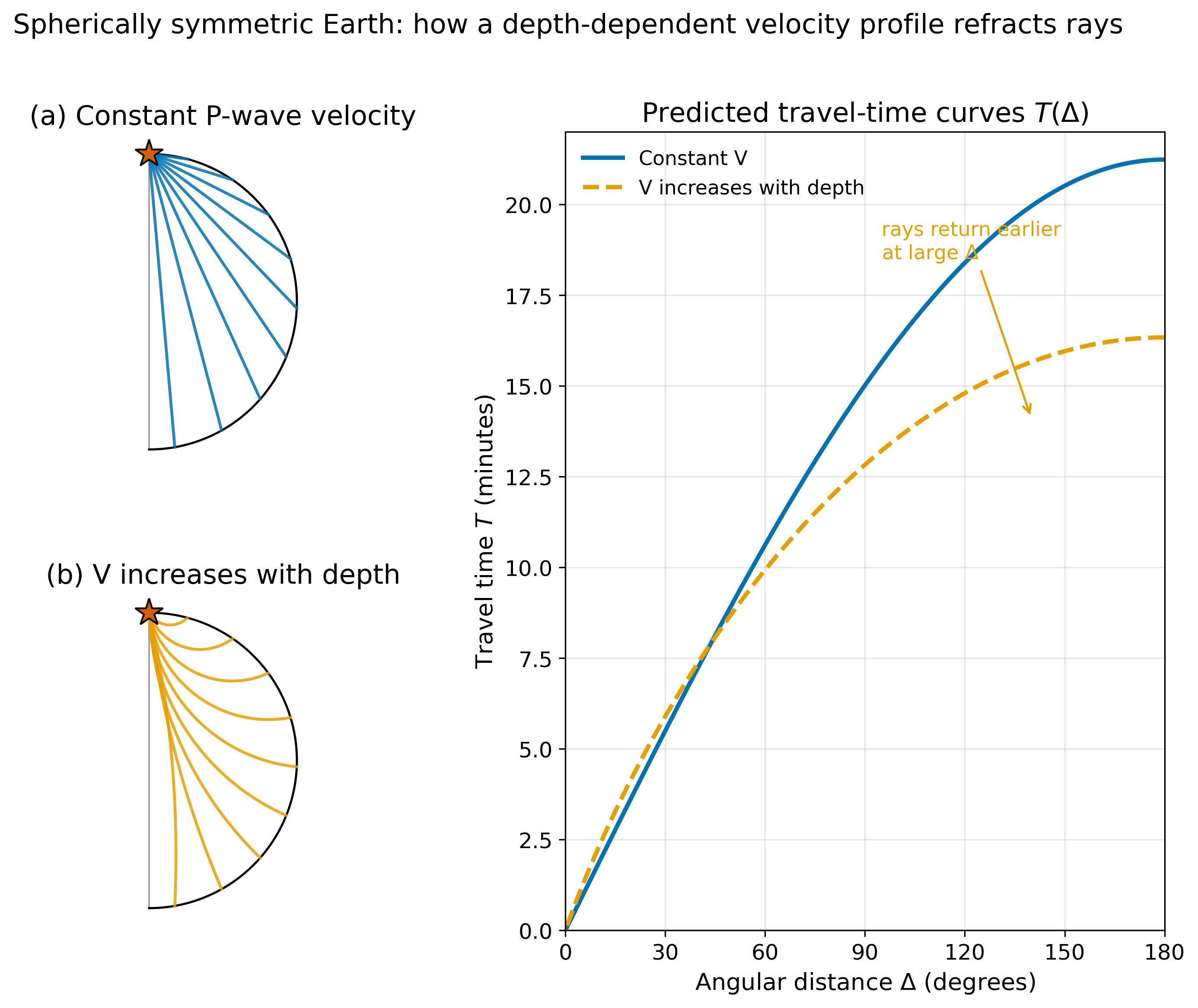
Fig. 43 straight blue ray paths (chords) from a source at the top to points along a half-circle, for a constant-velocity Earth. Bottom-left shows orange concave-up ray paths that turn at progressively greater depths for rays reaching larger epicentral distances, for a velocity- increasing-with-depth Earth. The right panel plots travel time T versus angular distance from 0 to 180 degrees; the solid blue constant-V curve is always above the dashed orange gradient curve at large distances, and an annotation arrow points to the orange curve labelled “rays return earlier at large Delta”. :width: 90%#

Ray paths and travel-time curves for two hypothetical Earths. In a constant-velocity Earth, rays travel in straight chords and the travel-time curve is the chord length divided by velocity. When velocity increases with depth, Snell’s law bends rays concave-up and they emerge at greater distance with shorter travel times.

The key takeaway: the shape of the \(T(\Delta)\) curve encodes the depth dependence of velocity. A seismologist who measures travel times from many earthquakes recorded at many stations and plots them on a single \(T(\Delta)\) diagram is, without yet writing any equations, already measuring the interior of the Earth.

3. The mathematical framework: travel time as an integral of slowness#

Along a ray path parametrised by arc length \(s\), the travel time is

(95)#\[T \;=\; \int_{\mathrm{source}}^{\mathrm{receiver}} \frac{ds}{V(\mathbf{r})} \;=\; \int_{\mathrm{source}}^{\mathrm{receiver}} u(\mathbf{r})\, ds,\]

where \(u = 1/V\) is the slowness. In a spherically symmetric Earth, the ray path depends only on radius, and the travel time for a ray that turns at radius \(r_p\) can be written explicitly as

(96)#\[T(p) \;=\; 2\,p\,\Delta(p) + 2 \int_{r_p}^{R}\!\sqrt{\eta^2(r) - p^2}\;\frac{dr}{r}, \qquad \eta(r) = r/V(r),\]

where \(p\) is the ray parameter (the analogue of the horizontal slowness in a flat Earth) and \(\Delta(p)\) is the angular distance travelled. You will not be asked to derive or apply this integral in this course; we cite it only so that you know the machinery exists and is numerically tractable. What matters pedagogically is the inverse: given a set of measured travel times \(T_i\) at known distances \(\Delta_i\), find the function \(V(r)\) that is consistent with them. Solving that inverse problem is what gives us the preliminary reference Earth model (PREM) in Section 7.

4. The forward problem: predicting shadow zones from a layered Earth#

A spherically layered Earth with a fluid outer core (no S-wave propagation; a sharp velocity decrease for P-waves at the CMB) makes two predictions that are qualitative enough for a student to check from first principles.

The S-wave shadow zone. S-waves cannot propagate through a fluid. Any S-ray that would have sampled the outer core is absorbed or converted at the CMB. From a shallow earthquake, the deepest mantle S-ray turns just above the CMB and emerges at \(\Delta \approx 103^\circ\). Beyond \(103^\circ\), no direct S-wave arrival can exist. The entire far hemisphere is an S-wave shadow.

The P-wave shadow zone. P-waves do propagate through the outer core — but at \(8.06\) km/s instead of the \(13.7\) km/s just above the CMB. The sudden velocity drop refracts descending rays strongly toward the vertical (Snell’s law with a low-velocity target layer), bending them far from where a no-core Earth would send them. The consequence is a ring, between roughly \(103^\circ\) and \(143^\circ\), where neither direct P nor refracted PKP arrives. Beyond \(143^\circ\), PKP emerges from the far side of the core.

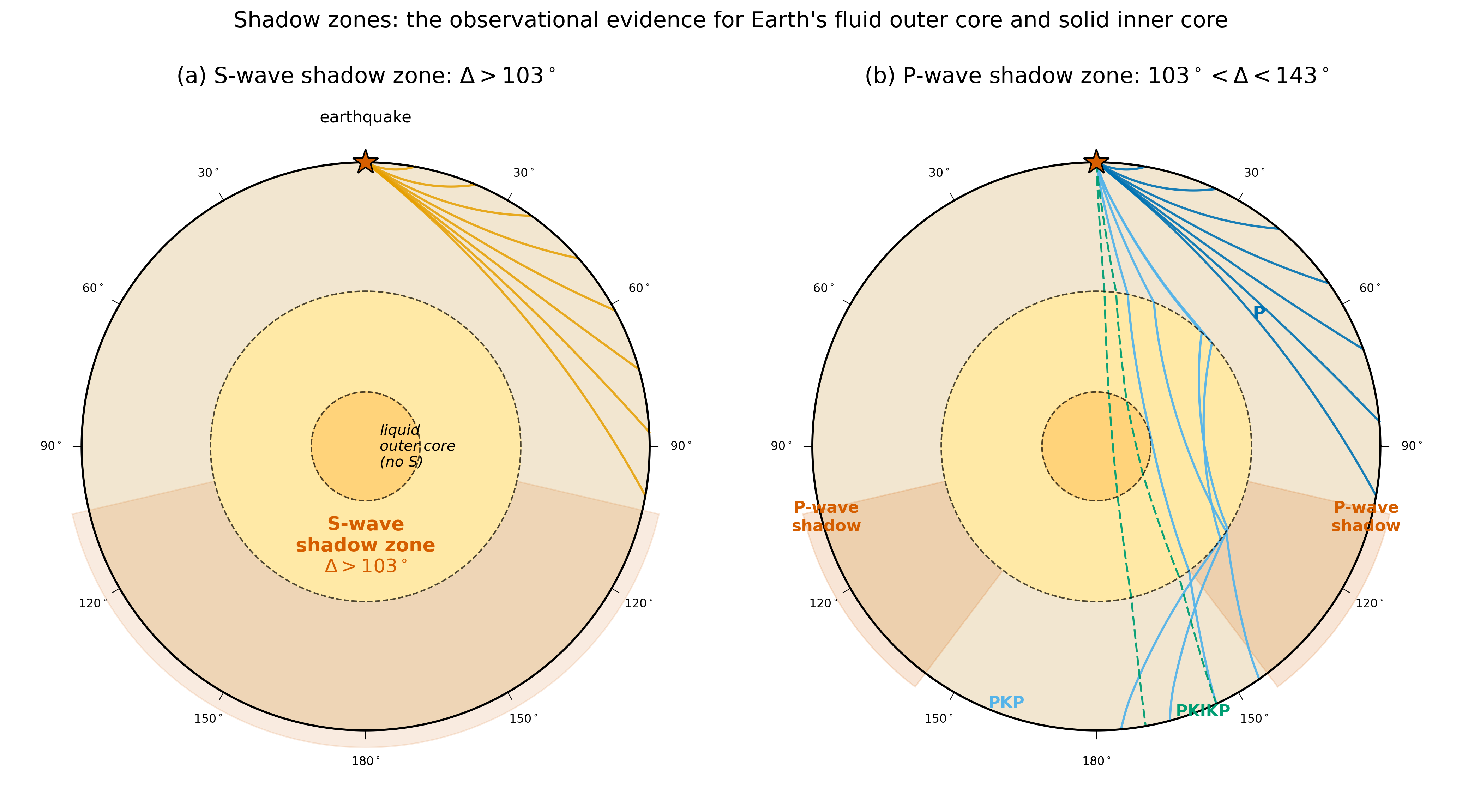
Two side-by-side schematic Earth cross-sections. Panel (a): — Fig. 44 S-wave shadow. Orange S-rays from a star-shaped source at the top of the Earth turn back inside the mantle and reach the surface only at angular distances less than 103 degrees. The surface arc from 103 degrees through the antipode at 180 degrees is shaded in vermilion and labelled “S-wave shadow zone”. The annotation inside the outer core reads “liquid outer core (no S)”. Panel (b): P-wave shadow. Blue P-rays turn in the mantle and reach the surface within 103 degrees; light-blue PKP rays refract into the outer core, traverse it along curved paths computed from AK135, and emerge at the surface beyond the PKP caustic at 143 degrees. Dashed green PKIKP rays pass through the outer core and continue through the solid inner core, emerging at distances near 155–175 degrees. The surface arc from 103 degrees to 143 degrees on each side is shaded in vermilion and labelled “P-wave shadow”. Angular distance ticks in 30-degree increments run from 0 to 180 on both sides of each panel. Both panels use the colorblind-safe Wong palette. :width: 100%#

Shadow zones are the direct observational signature of the fluid outer core. The 103° threshold is **geometric** — it is the angular distance at which a direct mantle ray just grazes the core-mantle boundary. Beyond 103° any direct ray must penetrate the core.

**S-wave shadow** (\(\Delta > 103^\circ\)): S-wave energy cannot propagate as a shear wave in the fluid outer core (\(\mu = 0 \Rightarrow \beta = \sqrt{\mu/\rho} = 0\)), so the S shadow extends from 103° all the way to the antipode.

**P-wave shadow** (\(103^\circ < \Delta < 143^\circ\)): P-wave energy refracts into the core (\(\alpha_\text{mantle} \approx 13.7\) km/s, \(\alpha_\text{outer\,core} \approx 8\) km/s; by Snell’s law the ray bends strongly toward the normal) and re-emerges as PKP at or beyond the PKP caustic near 143°, leaving a gap in the 103°–143° band.

The same kinematic boundary at the CMB combined with one constitutive fact — fluids carry no shear stress — explains both shadows.

**Reproducibility.** Ray paths in panel (b) use real obspy.taup AK135 ray tracing. The precise caustic position and PKP emergence distances depend on the radial velocity model; this figure uses AK135 (Kennett et al. 1995). Source: `assets/scripts/fig_11_shadow_zones.py`.

Oldham (1906) observed the S-wave shadow and inferred the fluid core. Gutenberg (1914) refined the depth estimate to \(\approx 2900\) km. Lehmann (1936) found a weak P-wave arrival inside the predicted P-shadow band at distances around \(150^\circ\)–\(160^\circ\) that could not be explained by the fluid-core model alone, and inferred a solid inner core at \(\approx 5150\) km depth. Three discoveries — each one a simple geometric argument from a missing or unexpected arrival on a seismogram — built the layered structure of the planet.

Key Equation — shadow-zone prediction

For a spherical Earth with mantle P-velocity increasing monotonically from \(V_P \approx 8\) km/s at the Moho to \(V_P \approx 13.7\) km/s just above the CMB, and an abrupt drop to \(V_P \approx 8.06\) km/s in the outer core, Snell’s law predicts:

\[ \Delta_{S\text{-shadow start}} \approx 103^\circ, \qquad 103^\circ \lesssim \Delta_{P\text{-shadow}} \lesssim 143^\circ. \]

These are numbers that students can derive themselves given the velocity contrast and the ray-parameter conservation rule \(p = r\sin i / V\). Lab 6 walks through this calculation.

Reasoning sketch — why \(p = r\sin i / V\) is the right invariant

In a flat-layered Earth, Snell’s law conserves \(\sin i / V\) at every interface. In a spherically symmetric Earth the geometry has changed: “horizontal” is no longer a single direction. What is preserved instead is the Bullen ray parameter

\[ p \;=\; \frac{r \sin i(r)}{V(r)} \;=\; \text{constant along a ray}, \]

where \(r\) is radius and \(i(r)\) is the angle between the ray and the local radial direction. Two facts make this work, and you should be able to argue both:

Spherical symmetry. Velocity depends only on \(r\); rotating the source–receiver geometry around Earth’s centre does not change the physics. Noether-style: a continuous symmetry implies a conserved quantity. Here the conserved quantity is the angular momentum-like product \(r\sin i / V\).
Turning condition. A ray turns where \(i = 90°\), i.e. where \(r/V(r) = p\). Plotting \(r/V(r)\) for AK135 makes the shadow-zone numbers visible: every \(p\) that maps onto the mantle part of the curve corresponds to a ray that emerges at \(\Delta < 103°\); the first \(p\) small enough to reach the CMB defines the 103° edge; rays that hit the velocity drop at the CMB refract steeply into the core and re-emerge as PKP beyond 143°.

The reasoning chain is: symmetry → conserved quantity → turning depth → emergence distance. Once internalised, every global travel-time diagnostic in this lecture and Lab 6 is a consequence.

5. The inverse problem: from global seismograms to a 1-D Earth#

Travel-time curves are assembled empirically. Global networks such as the IRIS Data Management Center and GEOSCOPE archive seismograms from thousands of earthquakes at hundreds of stations. When many seismograms are aligned by origin time and plotted against source-receiver distance, coherent arrival curves emerge for each body-wave phase. Figure Fig. 45 shows a modern computed version, using the AK135 reference Earth model (Kennett et al. 1995) as the interior structure and the obspy.taup ray-tracing package to calculate travel times.

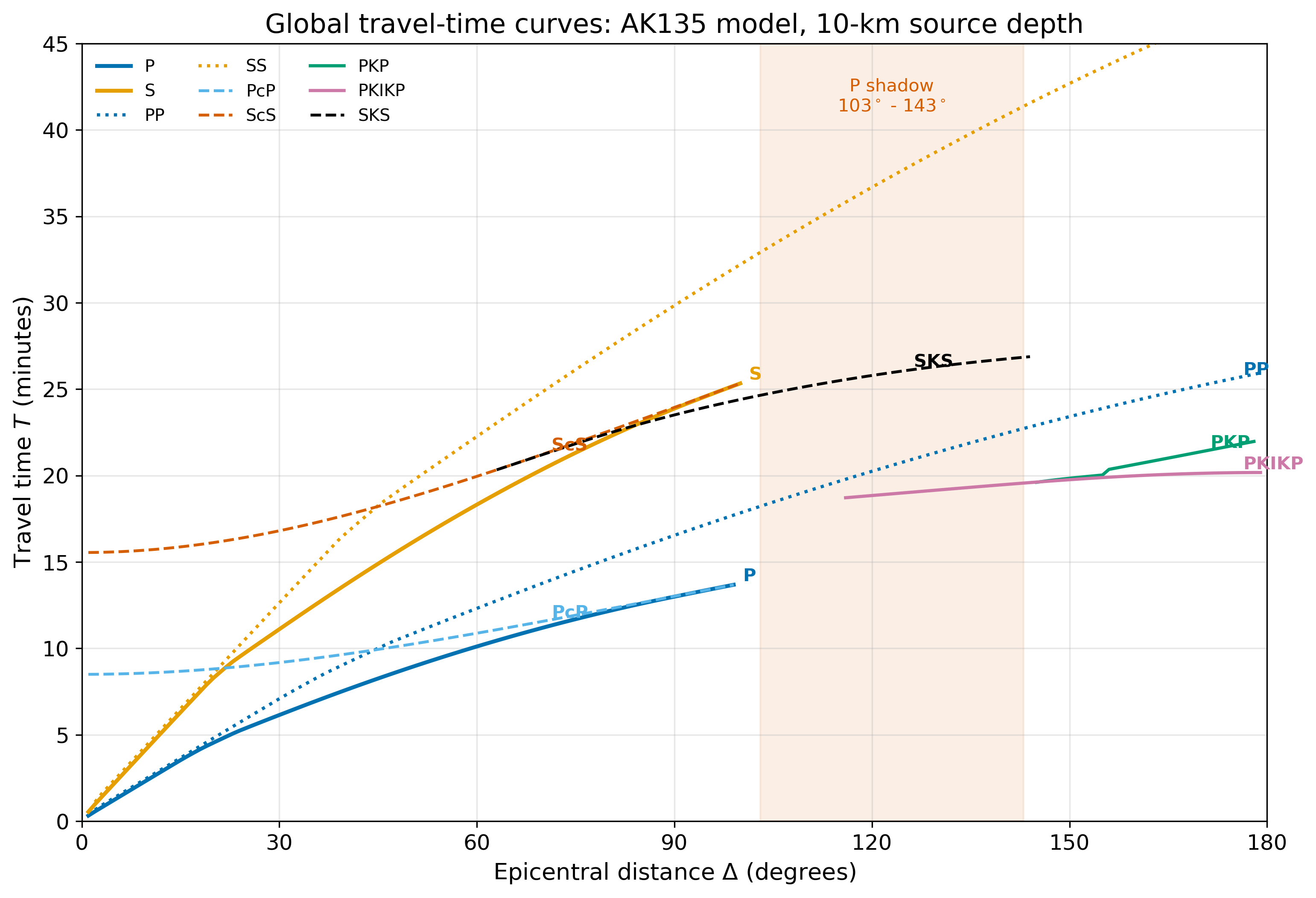
Global travel-time diagram plotting travel time in minutes on — Fig. 45 the vertical axis from 0 to 45 versus epicentral distance in degrees on the horizontal axis from 0 to 180. Curves for the phases P (solid blue), S (solid orange), PP (dotted blue), SS (dotted orange), PcP (dashed light blue), ScS (dashed red-orange), PKP (green), PKIKP (magenta) and SKS (dashed black) are plotted. A pale orange vertical band from 103 to 143 degrees is labelled “P shadow” and shows P and PP terminating at the left edge while PKP and PKIKP emerge at the right edge. Phase labels sit at the right ends of each curve. :width: 95%#

Global travel-time curves for the AK135 reference Earth model, computed for a 10-km-deep source using `obspy.taup`. Each curve is the forward prediction of a different phase. The shaded band marks the P-wave shadow zone: P and PP terminate at its left edge, and the core-refracted phases PKP and PKIKP emerge at its right edge. SKS appears near \(80^\circ\) where S-wave energy can convert to P at the CMB and back.

Reading this diagram is a fundamental skill. A student who can identify which travel-time branch corresponds to which phase, and who understands what part of Earth each phase has sampled, can interpret almost any global seismogram. Phase identification is also the foundation on which every higher-order seismology skill is built. Lab 6 puts this skill into practice using live IRIS data.

Phase naming convention

A single upper-case letter denotes a leg of the ray path. The conventions are: P = P-wave in the mantle; S = S-wave in the mantle; K = P-wave in the outer core; I = P-wave in the inner core; J = S-wave in the inner core. A lower-case c denotes reflection at the CMB, a lower-case i denotes reflection at the ICB. Thus PcP is a P-wave that descends through the mantle, reflects off the CMB, and returns through the mantle; PKIKP passes through mantle, outer core, inner core, outer core, and back through the mantle.

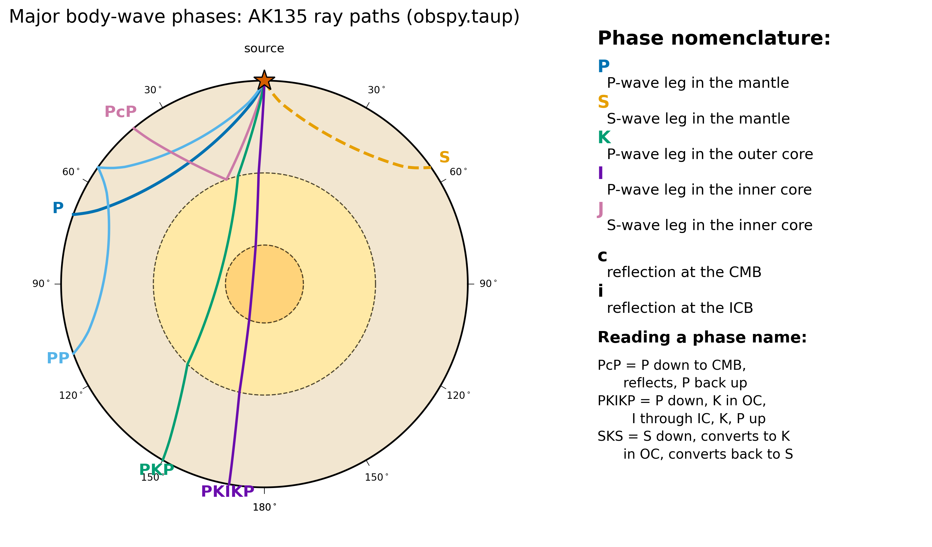
Left: cross-section of Earth with a source at the top and — Fig. 46 labelled ray paths for P (solid blue arcing through mantle to the right), S (dashed orange arcing through mantle to the left), PP (light blue, two concave arcs meeting at a surface reflection midway), PcP (pink, V-shape reflecting off the CMB), PKP (green, four-leg path refracting through the outer core), and PKIKP (dark purple, dashed, passing through mantle, outer core, inner core, outer core, and back through mantle). Tick marks in 30-degree increments from 0 to 180 on both sides. Right: phase-nomenclature key listing P, S, K, I, J, c, i with their meanings, and example readings for PcP, PKIKP, and SKS. :width: 98%#

The major body-wave phases and the naming convention that encodes their ray paths. Each segment of a phase name describes one leg of the journey through Earth’s interior.

6. A worked example: measuring the depth to the CMB#

Suppose we know the P-wave travel time for a direct mantle arrival at \(\Delta = 90^\circ\) is \(T_P \approx 12.8\) min = 768 s, and the PcP reflection time at the same distance is \(T_{PcP} \approx 13.4\) min = 804 s (both from AK135). The differential time \(T_{PcP} - T_P = 36\) s corresponds to the extra path travelled by PcP, which descends all the way to the CMB and back before returning to the same receiver. Order-of-magnitude estimation says that extra path is approximately \(2(d_{\mathrm{CMB}} - d_{\mathrm{turning\ depth\ of\ P}})\) divided by the average mantle P-velocity of \(\sim\) 11 km/s, so

\[ d_{\mathrm{CMB}} - d_{P\text{-turn}} \;\sim\; \tfrac{1}{2} \cdot 11 \; \mathrm{km/s} \cdot 36\;\mathrm{s} \approx 200\;\mathrm{km}. \]

Combined with the estimate that the direct P-ray at \(90^\circ\) turns near \(\sim 2700\) km depth, this places the CMB at roughly \(2900\) km. That is the Gutenberg discontinuity, and the crude estimate is within a few percent of the modern value of \(2891\) km.

7. The answer: the Preliminary Reference Earth Model (PREM)#

Three quarters of a century of global travel-time measurements, normal-mode observations, and mass-and-inertia constraints were inverted jointly by Dziewonski and Anderson (1981) to produce the Preliminary Reference Earth Model (PREM). PREM reports \(V_P\), \(V_S\), density \(\rho\), attenuation \(Q\), and transverse anisotropy as functions of radius. It remains the standard 1-D reference 45 years after publication, and every 3-D tomographic model published since is reported as a deviation from PREM or a close relative such as AK135.

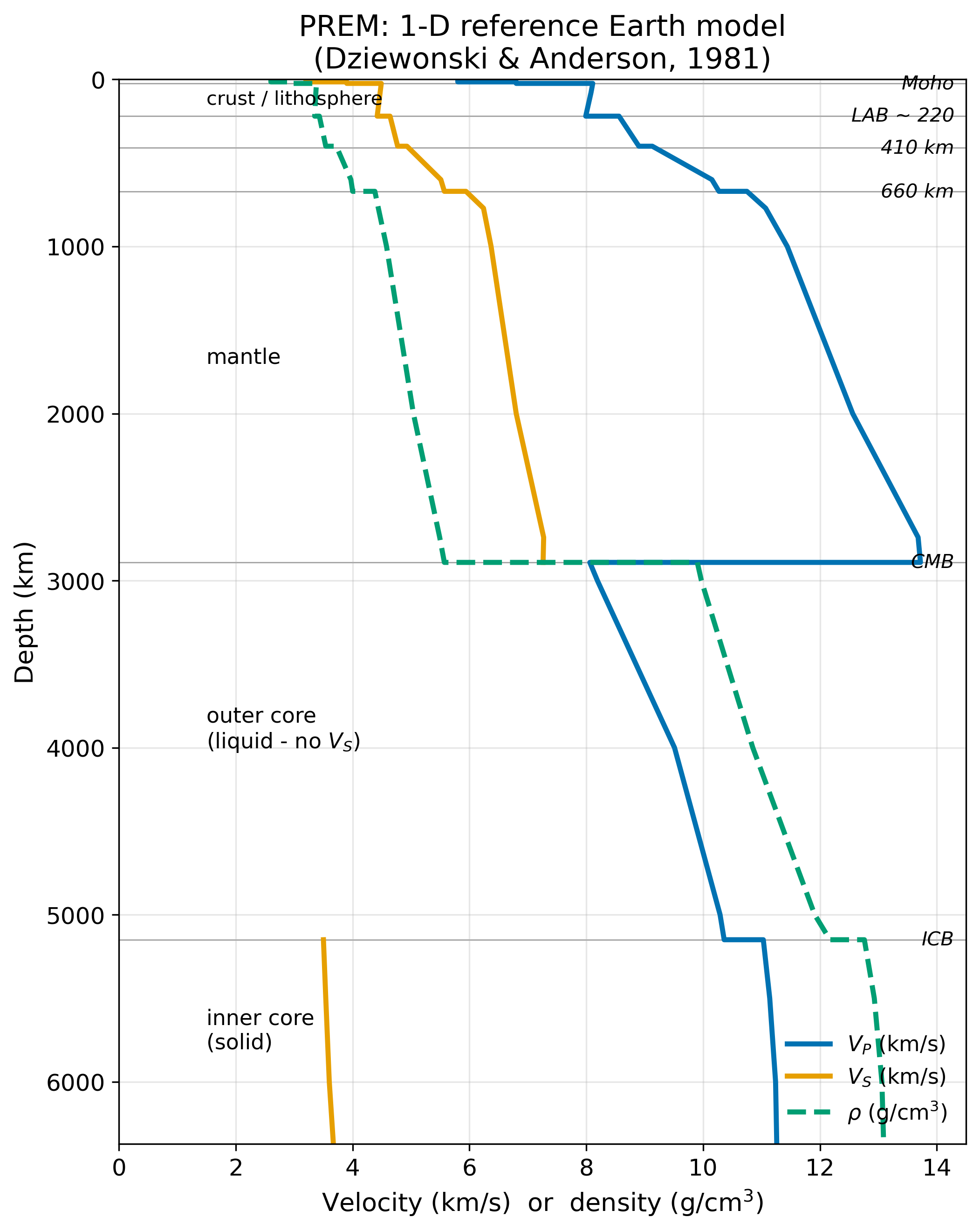
Fig. 47 the surface to 6371 km at Earth’s centre, and velocity or density on the horizontal axis from 0 to 14.5 km/s or g per cubic cm. Blue solid curve shows P-wave velocity Vp rising stepwise from 5.8 km/s at the surface through jumps at the Moho (24 km), 410 km, and 660 km, reaching 13.7 km/s just above the core-mantle boundary at 2891 km, dropping abruptly to 8.1 km/s across the CMB, then increasing through the outer core to about 10.3 km/s at the inner-core boundary at 5150 km where it jumps to about 11.0 km/s in the inner core. Orange solid curve shows S-wave velocity Vs, rising similarly through the mantle from 3.2 to 7.3 km/s, then dropping to zero in the outer core (a gap in the line) and reappearing at about 3.5 km/s in the solid inner core. Dashed green curve shows density, increasing from about 2.6 at the surface to about 13.1 g per cubic cm at Earth’s centre. Horizontal guide lines mark the Moho, LAB, 410, 660, CMB, and ICB; layer labels on the left identify crust and lithosphere, mantle, liquid outer core (with no Vs), and solid inner core. :width: 70%#

The Preliminary Reference Earth Model (PREM; Dziewonski and Anderson 1981). The three curves are \(V_P\) (blue), \(V_S\) (orange), and density (green dashed). Major discontinuities are annotated. The gap in the \(V_S\) curve across the outer core is the seismological signature of a liquid layer: shear waves cannot propagate. The jump in \(V_P\) at the inner-core boundary, together with the reappearance of \(V_S\) inside the inner core, indicates solid iron.

PREM is an inverse solution in the cleanest possible sense: an enormous number of observations (travel times of many phases at many distances, periods of free-oscillation eigenmodes, the mass and moment of inertia of the planet) are combined with a parametrisation of \(V_P(r)\), \(V_S(r)\), \(\rho(r)\) through several hundred parameters, and optimisation finds the profile that best fits all data jointly. The solution is non-unique; ten different radial profiles that differ by small oscillations can fit the same travel-time data to within their error. PREM was chosen because it is smooth and physically reasonable, not because it is the only profile consistent with the data. Lecture 12 will return to this point.

Reasoning prompt — why density needs separate data

Travel-time data of body waves constrain \(V_P(r)\) and \(V_S(r)\) but not \(\rho(r)\) directly: a P-wave travel time depends on \(V_P = \sqrt{(\kappa + \tfrac{4}{3}\mu)/\rho}\), so a \(\rho\) change can always be absorbed by a corresponding change in \(\kappa\) or \(\mu\). Density enters PREM through three independent constraints that body-wave times alone cannot supply:

Total mass \(M_\oplus = 5.972\times 10^{24}\) kg (from Newtonian gravity + the Moon’s orbit) sets \(\int_0^R \rho(r)\,4\pi r^2 dr\).
Moment of inertia \(I/M_\oplus R^2 \approx 0.3307\) (from precession and lunar laser ranging) sets the radial weighting of \(\rho(r)\) — a denser core lowers \(I/M R^2\).
Free-oscillation eigenfrequencies depend on the elastic moduli and on \(\rho\) through the equations of motion, breaking the \(\rho\)–modulus trade-off at specific depths.

Reasoning question to take to office hours: if we only had body-wave travel times (no mass, no moment, no normal modes), could we still prove the inner core is solid? Argue from the role \(V_S\) plays in the PKIKP raypath, then explain what we could not determine.

Reasoning prompt — what the shadow zone tells us, and what it doesn’t

The shadow zone proves the outer core is liquid (no \(V_S\) at any depth in the 103°–180° band) and bounds the core radius (the geometric 103° edge fixes where the CMB sits). It does not by itself prove:

The core is iron-rich (density argument from mass + moment).
The inner core is solid (Lehmann’s PKIKP energy in the gap; J-wave detections by Tkalčić & Pham 2018).
The inner core rotates differentially (decadal PKIKP residuals).

Distinguishing what a single observation constrains from what is layered on top of it through additional data is the central reasoning skill of whole-Earth seismology.

8. Connecting to Cascadia and the Pacific Northwest#

The travel-time curves and the PREM profile describe a spherically symmetric reference Earth — a useful zeroth-order model, but not literally the planet we live on. Three-dimensional deviations from PREM reveal the Juan de Fuca slab subducting beneath our feet, the mantle wedge that feeds the Cascade arc, and the plume tail beneath Yellowstone. Every time a Cascadia seismologist measures a teleseism arriving at a PNSN station, the first-arrival time is compared to the AK135 prediction; the residual, positive or negative by a few seconds, is a direct measurement of 3-D mantle structure beneath the station. This is the material of Lecture 12.

9. Research Horizon#

Modern whole-Earth seismology is moving beyond the 1-D reference picture in several directions.

Inner-core differential rotation. Cross-comparisons of PKIKP travel times from repeating earthquake sources recorded over decades (Song and Richards 1996; Tkalčić and Pham 2018) have identified small but resolvable inner-core rotation rates relative to the mantle. The most recent analysis of multi-decade PKIKP doublets reports annual-scale variability in both the rotation rate and the near-surface structure of the inner core (Vidale et al. [2025]), reframing the long-running “rotation vs. surface change” debate as a coupled, time-varying process rather than a steady differential rotation.
Comparative planetology. The NASA InSight mission placed a broadband seismometer on Mars in 2018 and recorded more than 1300 marsquakes through 2022. SKS-like converted phases have been used to image the Martian core, establishing that it is liquid and larger than previously thought (Stähler et al. 2021, https://doi.org/10.1126/science.abi7730). Apollo-era seismometers on the Moon similarly imaged a small lunar core (Weber et al. 2011, https://doi.org/10.1126/science.1199375).
CMB and inner-core boundary texture. Ultra-low velocity zones (ULVZs) and D″ phase transitions detected with ScS precursors and PKKP-diffracted phases are now being mapped globally, with implications for mantle plume anchoring (Cottaar and Lekić 2016).
AI-assisted global tomography. Machine-learning phase-picking (e.g., PhaseNet, Zhu and Beroza 2019, https://doi.org/10.1093/gji/ggy423; EQTransformer, Mousavi et al. 2020, https://doi.org/10.1038/s41467-020-17591-w) has increased global travel-time catalogs by one to two orders of magnitude over the past five years, enabling higher-resolution 1-D and 3-D models. The methodology is discussed in Lecture 12.

10. AI Literacy#

AI Literacy — Shadow Zone Epistemics (LO-7)

Prompt Lab. Ask a chat assistant: “Why does the S-wave shadow zone extend to 180° but the P-wave shadow zone only goes from 103° to 143°?” Then evaluate the response against Figure Fig. 44.

Common failure modes to watch for:

Attributing both shadows to absorption rather than distinguishing the two distinct mechanisms (fluid constitutive property for S; refraction geometry for P).
Confusing 103° geometry with the width of the P-shadow: 103° is set by the ray that grazes the CMB; the outer edge at 143° is set by the PKP caustic, a separate piece of physics.
Hallucinating velocity numbers: correct values are \(\alpha_\text{mantle} \approx 13.7\) km/s and \(\alpha_\text{outer\,core} \approx 8\) km/s just across the CMB; \(\beta_\text{outer\,core} = 0\).

The epistemic skill. Compare what the model says against the figure and against obspy.taup.TauPyModel('ak135'). Report numerical discrepancies explicitly and treat AI-generated shadow-zone explanations as drafts to cross-check, not authoritative answers.

AI Literacy — Phase-Name Epistemics (LO-7)

Prompt to try. “List the seismic phases that pass through Earth’s inner core and give their typical travel-time ranges for a teleseism at 150 degrees epicentral distance.”

What to check. A modern language model will readily produce a confident-sounding list: PKIKP, PKJKP, PKiKP, and perhaps others. Your task is to verify, independently, each claim the model makes. For each phase the model names, answer three questions: (i) is the phase name syntactically valid under the P/S/K/I/J/c/i convention? (ii) does the phase actually exist — i.e., has it been observed on real seismograms? (iii) is the travel-time range the model gives consistent with what obspy.taup.TauPyModel (ak135 or iasp91) returns for 150 degrees? Phase names like PKJKP and PKiKP are controversial — some have been claimed in the literature but never unambiguously confirmed. A model that reports them without flagging the controversy is hallucinating authority.

The epistemic skill. Never treat an AI-generated list of named scientific objects as a primary source. Cross-check against a first-principles tool (here, obspy.taup) and a peer-reviewed review paper. Report discrepancies as discrepancies, not as minor details to paper over.

11. Concept Checks#

[LO-11.1] If the Earth had a uniform P-wave velocity of \(V_P = 10\) km/s everywhere from surface to centre, what would the travel time be for a ray emerging at \(\Delta = 180^\circ\)? Compare to the actual PKIKP time (about 20 minutes) and explain the sign of the difference.
[LO-11.2] A seismogram records a clear first arrival at \(T = 7\) min for a known earthquake. You also identify an S-like arrival at \(T = 13\) min. Using Figure Fig. 45, estimate the epicentral distance. What phases would you expect to see next, and at what times?
[LO-11.3] Lehmann’s 1936 discovery of the inner core rested on observing P-wave energy inside the predicted P-wave shadow zone. Explain, in terms of Snell’s law, why a solid inner core with \(V_P > V_P\)(outer core) would produce such arrivals. What would the PKIKP travel-time curve look like if the inner core did not exist?
[LO-11.3 — reasoning chain] Suppose a future probe of an exoplanet records body-wave travel times that show no S-wave shadow zone at any distance, but a P-wave shadow at \(\sim 110^\circ\)–\(140^\circ\). What can you infer about that planet’s interior, and what can you not infer? Build the argument step by step from the shadow-zone reasoning of Section 4.
[LO-11.2 — quantitative reasoning] Two stations record the same earthquake at \(\Delta = 60^\circ\) and \(\Delta = 95^\circ\). Sketch how the Bullen ray parameter \(p = r\sin i / V\) differs between the two rays, predict which ray turns deeper, and explain why the deeper ray has the smaller \(p\). Use this to argue why the slope of the global \(T(\Delta)\) curve is monotonically decreasing with distance up to \(\sim 100^\circ\).

12. Connections#

Previous lectures. This lecture reuses Snell’s law (Lecture 3) and the concept of the forward/inverse problem (Lecture 4).
Companion lab. Lab 6 asks you to use obspy to download three real teleseisms recorded at IRIS-network stations, to pick the arrival times of the major phases, and to compare to AK135 predictions. The AI Literacy component of Lab 6 critically evaluates ML-based phase pickers against manual picks.
Next lecture. Lecture 12 takes the residuals — the observed-minus-predicted travel times — and uses them as data to invert for 3-D structure. The forward problem is the same one that built PREM; the twist is that the model \(\mathbf{m}\) now represents cell-by-cell velocity perturbations rather than a smooth radial profile.


Course LOs addressed	LO-2, LO-3, LO-5, LO-7
Learning outcomes practiced	LO-OUT-B (interpret travel-time curves), LO-OUT-C (explain physical reasoning from shadow zones), LO-OUT-E (evaluate 1-D Earth models)
Prior lectures	Lectures 3–4 (Snell’s law, ray-wavefront duality, slowness integral), Lecture 10 (forward/inverse problem framing)
Next lecture	Lecture 12 — Seismic Tomography
Lab connection	Lab 3: students compute AK135 travel times with obspy.taup and compare to observed phase picks
Discussion connection	Discussion 6: How shadow zones led to discovery — evaluating historical claims from first principles