Earthquake Phenomena I — Records, Phases, and Location

Earthquake Phenomena I — Records, Phases, and Location#

Prerequisites#

Before reading this lecture, students should be comfortable with the seismic-wave types introduced in Lectures 3–5 — body waves (P and S) and surface waves (Rayleigh and Love) — and with the elastic-wave velocities \(V_P\) and \(V_S\) in a Poisson solid. The mathematics of forward and inverse problems introduced in the refraction and tomography lectures (Lectures 6, 7, 12) carries over directly: the location problem is the same kind of problem with a different physical observable.

1. The framing question: where did the earthquake happen, and how do we know?#

The Pacific Northwest sits above one of the most consequential subduction zones in the world. Off the coast of Washington and Oregon, the Juan de Fuca plate is being thrust beneath North America at the Cascadia subduction zone. The plate interface is locked: it has not produced a great earthquake in the instrumental record, but paleoseismic and tsunami evidence date the last megathrust rupture to 26 January 1700, with a magnitude estimated near \(M_w\) 9. The shaking from the next such event will be felt across an area larger than the United Kingdom.

Between those very rare megathrust events, the Pacific Northwest experiences hundreds of smaller earthquakes every month — shallow crustal events in the North American plate, deeper intra-slab events within the descending Juan de Fuca slab, volcanic-tectonic events under Mount Rainier and Mount St. Helens, and slow-slip / tremor episodes that recur on a roughly 14-month cycle along the deeper portion of the plate interface. The Pacific Northwest Seismic Network (PNSN), operated jointly by the University of Washington and the University of Oregon, records these events on a network of broadband seismometers, strong-motion accelerometers, and increasingly on borehole and ocean-bottom instruments.

The fundamental question for everything that follows is mechanical: an earthquake is a sudden frictional slip on a quasi-planar fault surface within the Earth, releasing accumulated elastic strain energy as radiated seismic waves. The event itself is hidden — typically several to tens of kilometers below the surface, on a fault plane no observer will ever see directly during rupture. Yet from the wiggles recorded on instruments at the surface, modern seismology routinely determines where an event occurred, when it began, how big it was, and what kind of motion produced it. This lecture concerns the first two of those questions, which together constitute the earthquake-location problem: given arrival-time picks at a network of stations, infer the four coordinates \((x_0, y_0, z_0, t_0)\) that specify the hypocenter and origin time.

Schematic block diagram showing a near-vertical fault plane (dashed) cutting from depth to the surface, with a focus marker (orange star) at the centre and concentric blue wavefronts radiating outward. The epicenter (blue circle) sits directly above the focus on the ground surface; the focal depth, h, is annotated as the vertical separation. A small fault scarp is shown where the fault breaks the surface. 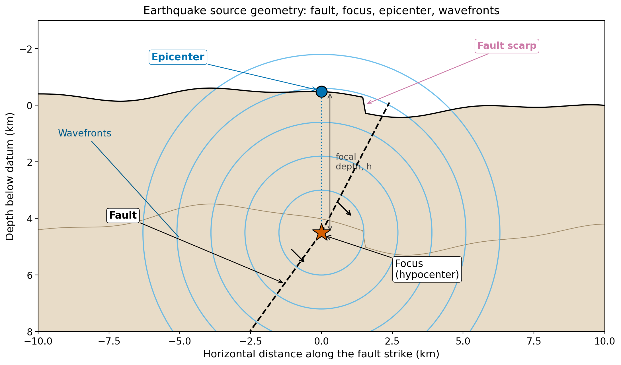— Fig. 57 Source geometry of an earthquake. The **focus** (or **hypocenter**) is the point at depth where rupture initiates; the **epicenter** is its vertical projection to the surface. The **focal depth** \(h\) is the vertical distance between them. Wavefronts spread outward through the Earth and reach instruments at the surface as the seismic waves whose anatomy is the subject of this lecture.#

2. The physics: a seismogram records P, S, and surface waves in time order#

Three pieces of physics that have already been developed in this course combine to make earthquake location possible.

The first is the decomposition of an elastic disturbance into compressional and shear modes. In a Poisson solid the two body-wave speeds satisfy \(V_P / V_S = \sqrt{3} \approx 1.73\), with \(V_P\) the larger. P-waves and S-waves leave a common source at the same instant, but their differing speeds cause them to separate in time as they propagate. The S-minus-P time at any station is therefore a measure of the distance traveled.

The second is Huygens’ principle and the spreading wavefront. From a compact source, an isotropic medium broadcasts spherical wavefronts in all directions. In the far field, geometric spreading reduces body-wave amplitudes as \(1/r\) and surface-wave amplitudes as \(1/\sqrt{r}\), but the arrival times are governed by the integral of slowness along the ray path — not by amplitude. This is what allows location to be cast as a problem about times, not amplitudes.

The third is the existence of a free surface. The Earth is bounded above by a stress-free interface that converts a fraction of the body-wave energy reaching it into surface waves — Rayleigh waves with elliptical retrograde particle motion in the vertical plane, and Love waves with horizontal transverse motion. Surface waves travel along the surface at \(V_R \approx 0.92\, V_S\), slower than body waves; they always arrive after the direct P and S phases at any teleseismic distance. The same free surface is responsible for the depth phases (pP, sP, sS) on which teleseismic depth determination depends.

A two-panel figure. Top panel is a cross-section of the Earth showing a focus star at 8 km depth, a dashed fault, four stations on the surface at horizontal distances of 20, 50, 90, and 140 km, and three concentric wavefronts radiating from the focus — a P wavefront (blue), an S wavefront (orange dashed), and a surface-wave streak (pink) along the surface. The static frame is captured at t = 11.8 s, when the P wavefront has reached about 71 km, the S wavefront 41 km, and the surface wave about 11 km from the epicenter. Bottom panel is a record section showing four traces stacked vertically; the trace for station S1 (closest) is fully developed with P, S, and surface-wave onsets marked, S2 has just received a P arrival, and S3 and S4 are still flat. Linear travel-time guides connect the P, S, and surface-wave arrivals across stations. 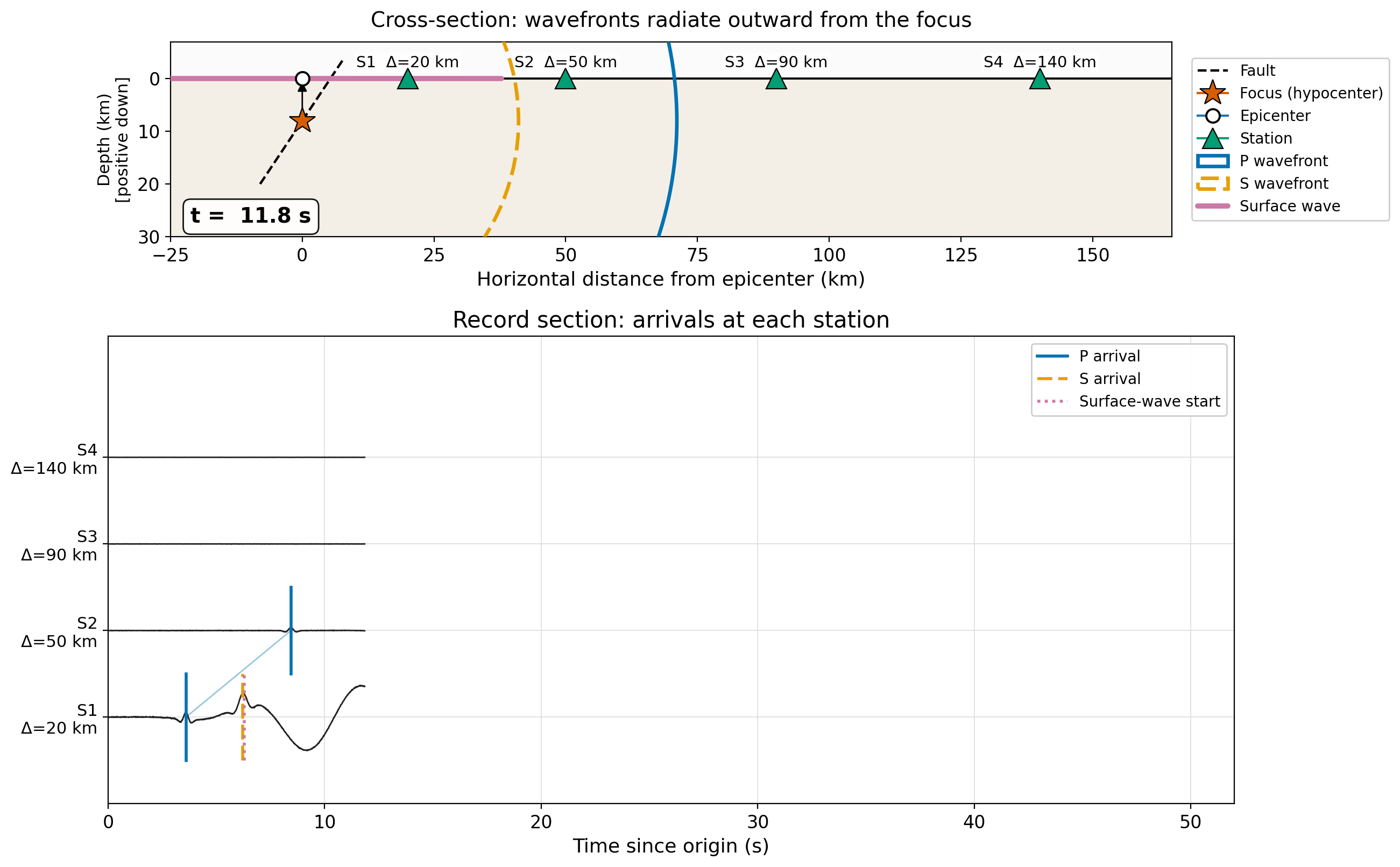— Fig. 58 Wave propagation from a focus at 8 km depth to four stations at increasing distance. Body-wave velocities \(V_P = 6.0\) km/s and \(V_S = V_P / \sqrt{3}\); surface-wave velocity \(V_R \approx 0.92\, V_S\). The three wavefronts spread outward at distinct speeds, producing arrivals in P → S → surface order at every station. The S-minus-P time grows linearly with distance, while the surface-wave delay relative to P grows still faster. The animated version of this figure (`fig_record_section_animation.gif`) shows the full evolution from \(t = 0\) to \(t \approx 50\) s.#

Key physical insight

The same source emits P, S, and surface waves at the same instant. The reason different stations record them at different times — and the reason a single station can convert a phase pair into a distance — is that the velocities are different and well-known. Earthquake location is fundamentally an exercise in unwrapping time differences using a known velocity model.

3. The mathematical framework: travel times as a forward operator#

Notation

Symbol	Meaning	Units
\((x_0, y_0, z_0)\)	Hypocenter coordinates (east, north, depth)	km
\(t_0\)	Origin time of the rupture	s
\(\mathbf{x}_i = (x_i, y_i, z_i)\)	Coordinates of the \(i\)-th station	km
\(T_P^{(i)},\ T_S^{(i)}\)	Observed P and S arrival times at station \(i\)	s
\(V_P,\ V_S,\ V_R\)	P-wave, S-wave, and Rayleigh-wave velocities	km/s
\(D_i\)	Hypocentral distance from source to station \(i\)	km
\(\Delta_i\)	Epicentral (surface) distance to station \(i\)	km
\(h\)	Focal depth	km
BAZ	Back-azimuth: direction from station to source	deg, clockwise from N

3a. The travel-time forward model

For a homogeneous, isotropic half-space and straight-line ray paths, the predicted P-wave arrival time at station \(i\) from a source at \((x_0, y_0, z_0, t_0)\) is

(106)#\[ T_P^{(i)\,\mathrm{pred}} \;=\; t_0 \;+\; \frac{1}{V_P}\,\sqrt{(x_i - x_0)^2 + (y_i - y_0)^2 + (z_i - z_0)^2}. \]

The predicted S-wave arrival time has the same form with \(V_P\) replaced by \(V_S\):

(107)#\[ T_S^{(i)\,\mathrm{pred}} \;=\; t_0 \;+\; \frac{1}{V_S}\,\sqrt{(x_i - x_0)^2 + (y_i - y_0)^2 + (z_i - z_0)^2}. \]

In a real Earth, the square-root expression is replaced by a travel-time integral along a ray path that bends through depth-varying velocity structure. The conceptual shape of the problem is the same, but the forward model becomes a non-linear functional of the source coordinates.

3b. The S-minus-P relation: distance from a single station

Subtracting equation (106) from (107), the origin time \(t_0\) cancels and the source-station distance \(D_i\) falls out as

(108)#\[ T_S^{(i)} \;-\; T_P^{(i)} \;=\; D_i \left( \frac{1}{V_S} - \frac{1}{V_P} \right). \]

Rearranging,

(109)#\[ \boxed{\;\;D_i \;=\; \frac{V_P\, V_S}{V_P - V_S}\,\bigl(T_S^{(i)} - T_P^{(i)}\bigr)\;\;} \]

Key Equation: S-minus-P distance

A single station, with a known crustal velocity model, converts a measured \(T_S - T_P\) time into a hypocentral distance \(D\). For typical continental crust \(V_P = 6.0\) km/s, \(V_S = 3.46\) km/s, the prefactor in equation (109) evaluates to \(V_P V_S / (V_P - V_S) \approx 8.2\) km/s. This is the origin of the textbook rule of thumb that the distance in kilometres is approximately eight times the S-minus-P time in seconds.

A horizontally laid-out single-component seismogram covering 32 minutes after the origin time. Shaded background colours partition the trace into four windows from left to right: a grey 'pre-event noise' window, a pale-blue 'P alone' window starting at the P onset at 9 minutes, a pale-orange 'P + S' window starting at the S onset at 16.5 minutes, and a pale-pink 'P + S + surface waves' window starting at the surface-wave onset at 25 minutes. Vertical lines mark each onset in matching colours. A double-headed arrow between the P and S onsets is annotated 'T_S − T_P ≈ 7.5 min'. The trace shows a small, short P pulse, a larger lower-frequency S pulse, and a long dispersive surface-wave train of largest amplitude. 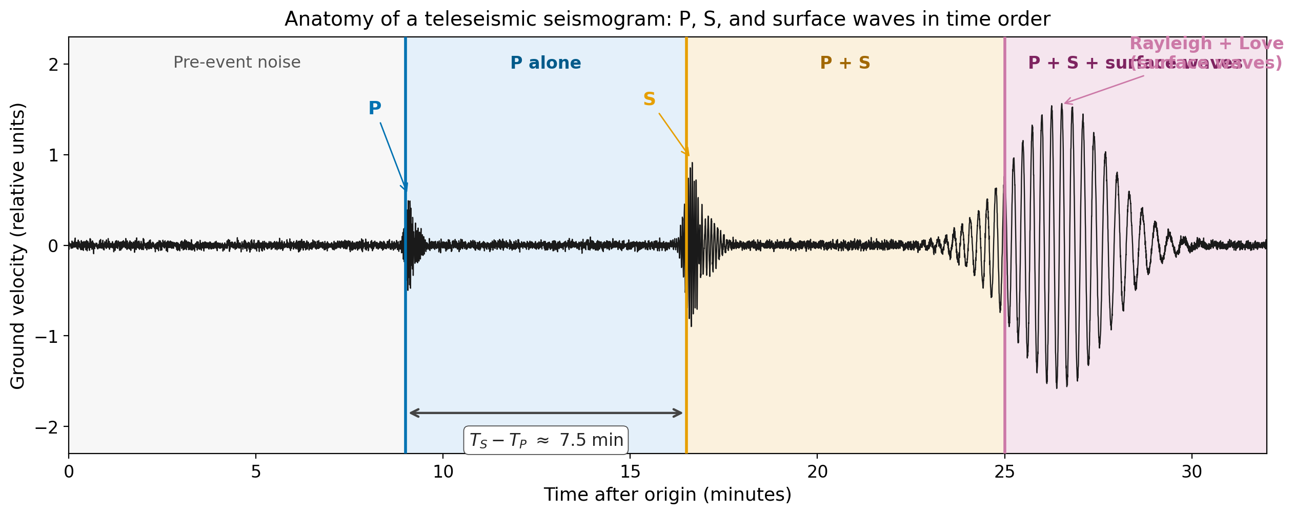— Fig. 59 Anatomy of a teleseismic seismogram. The three principal arrivals appear in time order: a short, high-frequency P pulse first; a longer, lower-frequency S pulse next; and a long-period, dispersive surface-wave train of largest amplitude last. The interval \(T_S - T_P\) — read directly off the record — is the diagnostic measure that converts to hypocentral distance via equation (109).#

A line plot of S-minus-P time on the vertical axis (0 to 50 seconds) versus hypocentral distance on the horizontal axis (0 to 200 km). Three straight lines through the origin are shown for three crustal velocity scenarios: a steep blue solid line for sedimentary basin (V_P=3.0, V_S=1.7) with slope 0.255 s/km; a medium orange dashed line for average crust (V_P=6.0, V_S=3.46) with slope 0.122 s/km; and a shallow green dash-dotted line for lower crust (V_P=7.0, V_S=4.0) with slope 0.107 s/km. A worked-example marker shows that a 6-second S-minus-P time in average crust corresponds to a hypocentral distance of about 49 km. A box at upper right reads 'Rule of thumb (avg. crust): r ≈ 8(T_S − T_P)'. A banner above the plot displays the equation T_S − T_P = r(1/V_S − 1/V_P), which rearranges to r = V_P V_S /(V_P − V_S) · (T_S − T_P). 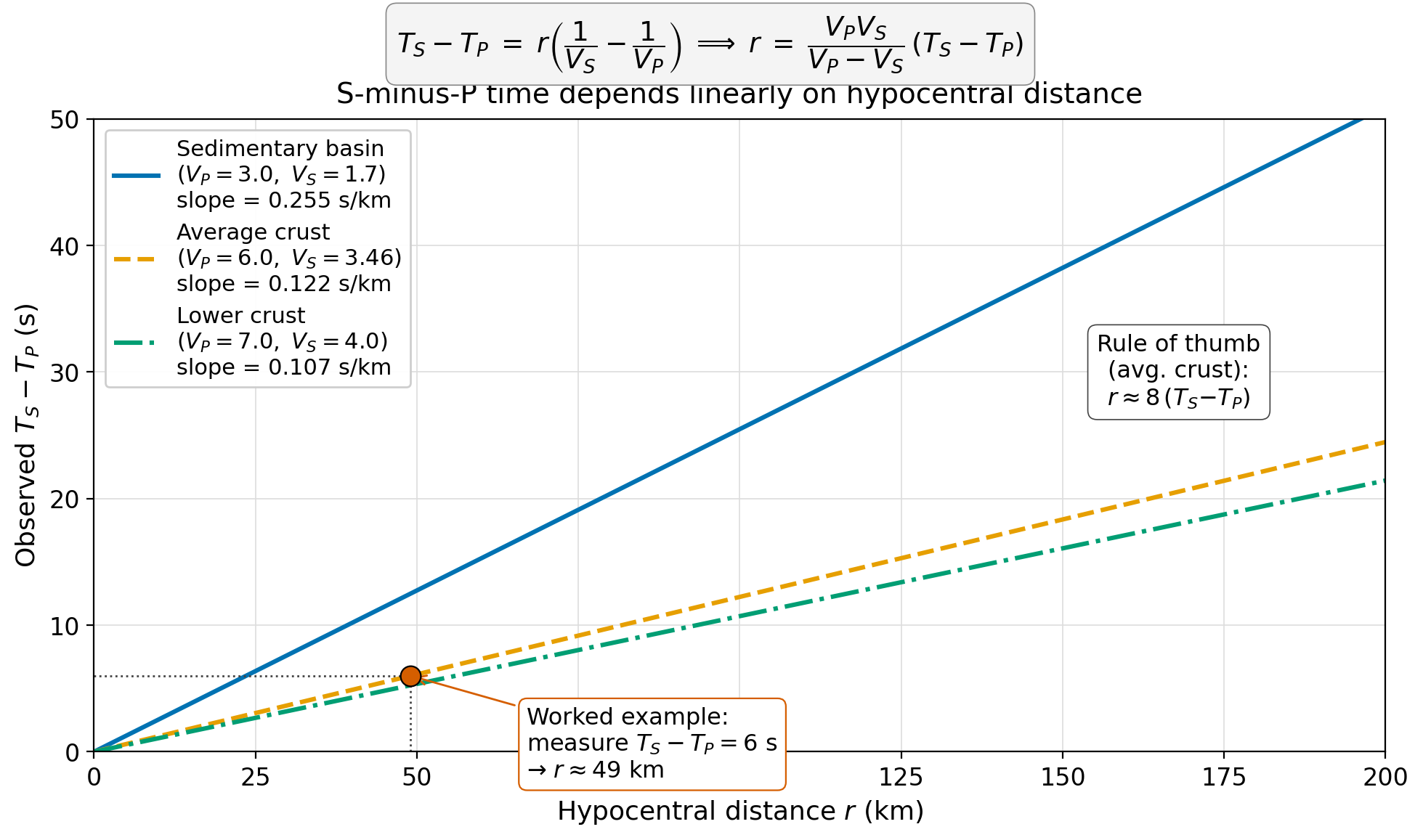— Fig. 60 Hypocentral distance as a linear function of \(T_S - T_P\) for three crustal velocity scenarios. Slower velocity contrasts (sedimentary basins) produce steeper slopes — a small misjudgment of the appropriate velocity model translates into a large distance error. The choice of velocity model is therefore a *prior assumption* that must be made explicit in any single-station distance estimate.#

3c. Single-station back-azimuth from polarization#

A single three-component station can also constrain the direction to the source through P-wave polarization. Because P-wave particle motion is parallel to the propagation direction, the first-motion amplitudes on the East and North horizontal components determine the azimuth in the horizontal plane:

(110)#\[ \mathrm{AZI} \;=\; \arctan\!\left(\frac{A_E}{A_N}\right). \]

The vertical-component first-motion polarity disambiguates the inherent \(180°\) ambiguity of the arctangent: an upward first motion (\(A_Z > 0\)) implies the source is in the same horizontal direction as \((A_E, A_N)\), while a downward first motion implies the opposite direction. The combination of \(D_i\) and BAZ from a single station nominally locates the epicenter — but in practice, the polarization estimate is noisy and the local velocity structure beneath the station distorts the apparent direction. Single-station locations are useful as a first guess; routine catalog locations always use multiple stations.

Two-panel figure. Left panel shows three first-motion seismogram segments stacked vertically — a blue trace labeled N with peak amplitude A_N=0.85, an orange trace labeled E with A_E=0.45, and a green trace labeled Z with A_Z=0.92 (up). A vertical dashed line marks the common P arrival time. Right panel is a compass rose with N at top, E to the right; a green station triangle sits at the centre. A vermilion arrow points from the station up and to the right at about 28 degrees east of north, labeled BAZ = 28°, with a callout 'To source (epicenter)'. A box at bottom reads 'BAZ = arctan(A_E/A_N) + 180° if Z is downward'. 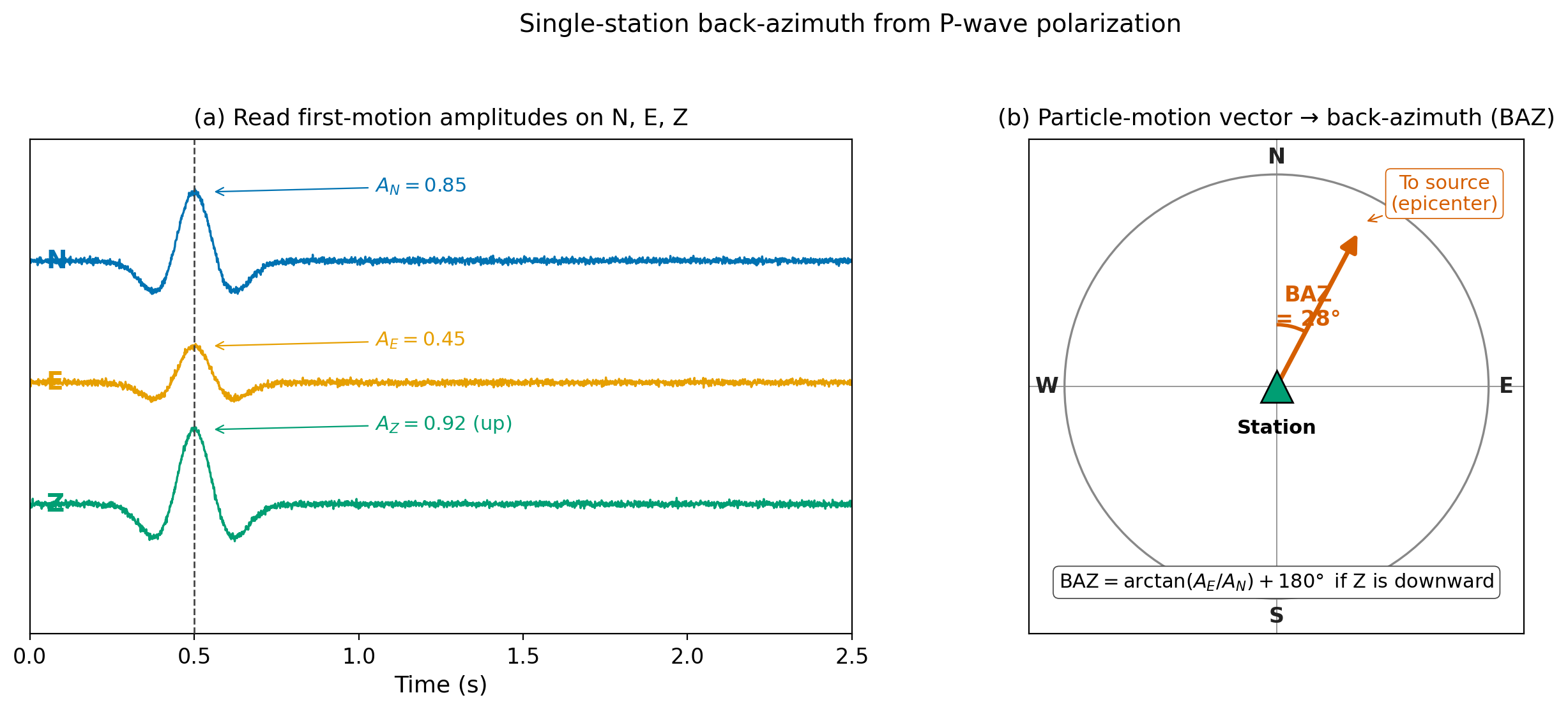— Fig. 61 Single-station back-azimuth from P-wave first-motion polarization. The horizontal particle-motion vector \((A_E, A_N)\) points either toward or away from the source depending on the vertical-component polarity.#

3d. Triangulation: the multi-station epicenter#

With three or more stations, each S-minus-P time defines a circle of constant hypocentral distance on the surface. Taking the focal depth as a known quantity (or assuming surface focus for a first guess), the epicenter must lie on the intersection of these circles. Three circles in general position intersect at a single point; with picking errors and an imperfect velocity model the circles bound a small residual region near the true epicenter. This residual region is what the inverse problem in section 5 minimizes.

Two-panel map view. Both panels show three green station triangles labelled S1, S2, S3 at different positions, with circles of distinct colours centered on each station and an orange star marking the true epicenter at the origin. In panel (a), with perfect picks, all three circles intersect cleanly at the epicenter and a callout reads 'Single intersection = epicenter'. In panel (b), with realistic picking errors, the circles no longer intersect at one point but bound a small residual region near the true epicenter; a callout reads 'Residual region (picking + velocity errors)'. 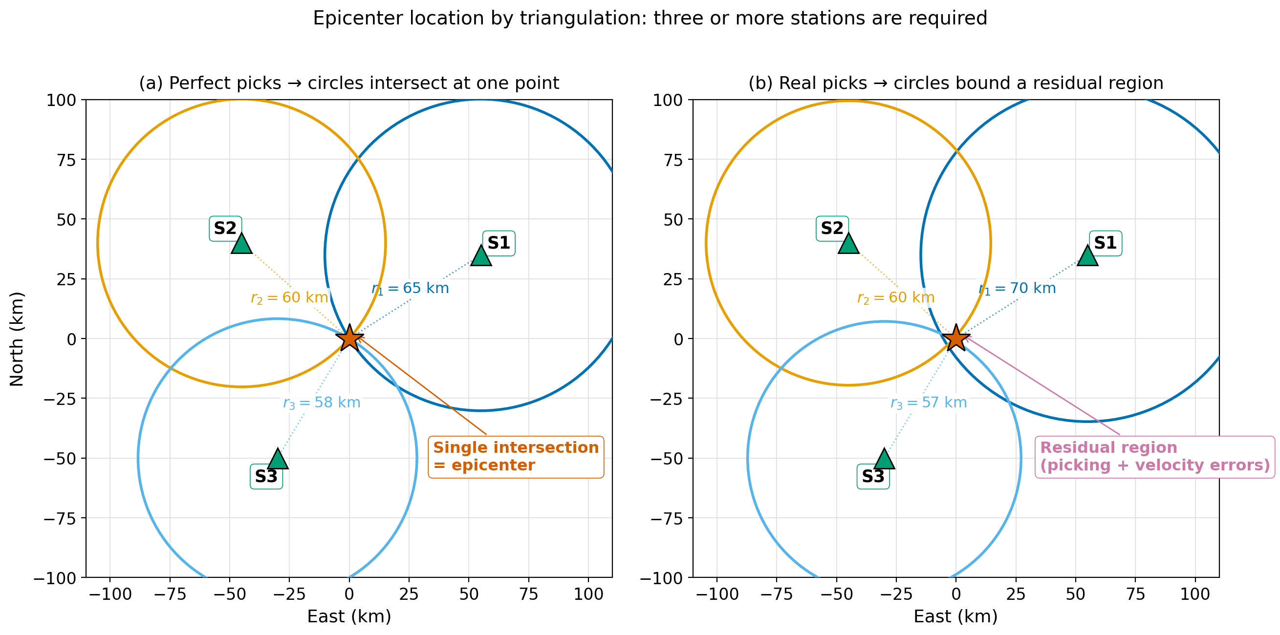— Fig. 62 Epicenter location by triangulation. (a) With perfect picks and perfect velocity model, three circles intersect at one point. (b) With realistic picking errors and an imperfect velocity model, the circles bound a small residual region — the inverse problem of section 5 finds the source position that minimizes the sum of squared residuals.#

3e. Resolving focal depth#

The fourth coordinate, the focal depth \(z_0\), is geometrically the hardest to recover. Two complementary methods are used in different distance regimes.

At local distances — a station within roughly \(\Delta \lesssim h\) of the epicenter — the propagation path is essentially straight, and the right triangle formed by the focal depth, the epicentral distance, and the hypocentral distance gives

(111)#\[ h \;=\; \sqrt{D^2 - \Delta^2}. \]

This requires that at least one station be close enough that \(\Delta\) and \(h\) are comparable, so the angle subtended at the source is large.

At teleseismic distances, where the station lies many thousands of kilometres from the source, the rays from the focus to the receiver all approach at similar steep takeoff angles, and the direct P arrival time alone is nearly insensitive to focal depth. The diagnostic is then the depth phase pP — a P-wave that leaves the source upward, reflects once off the free surface directly above the source, and then travels to the receiver. The differential time

(112)#\[ \Delta t_{pP} \;=\; t_{pP} - t_P \]

depends almost entirely on the focal depth, with a sensitivity of roughly \(0.4\) s per kilometre of depth in typical mantle structure.

Two-panel figure. Left panel shows a right triangle in cross-section with the epicenter at the origin, a station 13 km to the east on the surface, and a focus star at 8 km depth directly below the epicenter. The vertical leg is labelled h (focal depth), the horizontal leg labelled Δ (epicentral distance), and the hypotenuse labelled D (hypocentral distance). A box displays h = sqrt(D^2 − Delta^2). Right panel is a schematic Earth-quadrant cross-section to a depth of 600 km and an epicentral distance of 1100 km. A focus star sits at 200 km depth. A blue curved ray (direct P) descends from the focus to a station triangle at the right end. An orange ray (pP) leaves the source upward, reflects at the free surface 25 km from the epicenter, and then follows a path nearly parallel to the direct P ray to the same station. A small inset seismogram below shows two pulses separated by an interval labelled t_pP − t_P. 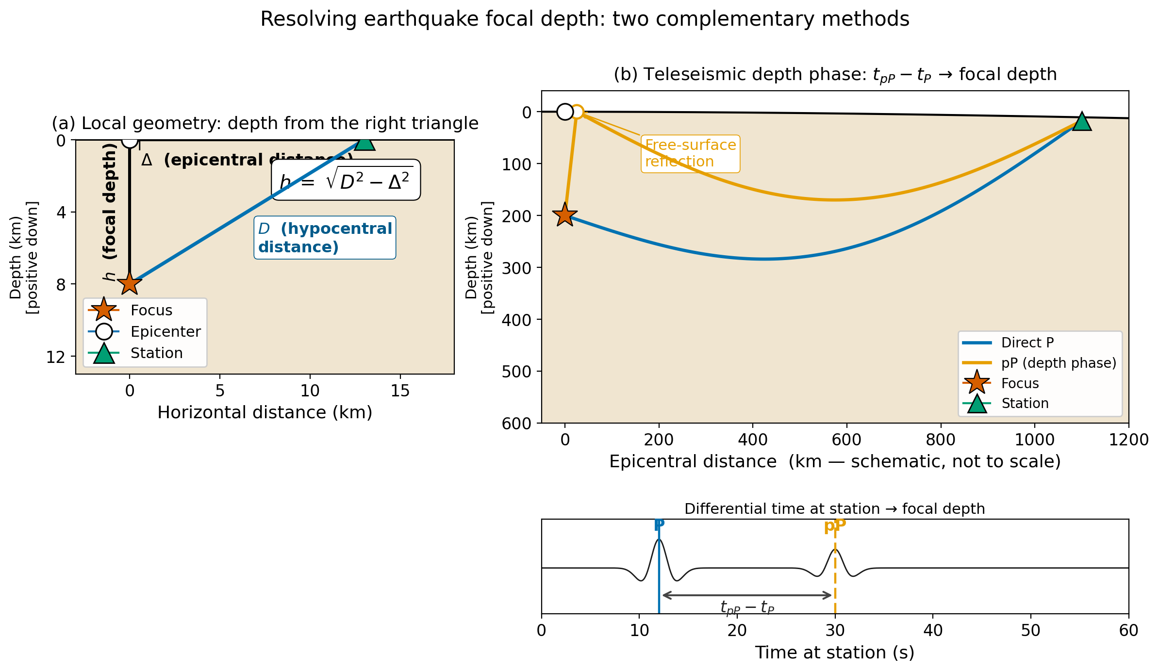— Fig. 63 Focal-depth determination. (a) At local distances the right triangle of focus, epicenter, and station gives the depth directly. (b) At teleseismic distances the depth phase pP — which reflects once at the free surface above the source — is separated from the direct P arrival by a time that depends almost entirely on focal depth.#

4. The forward problem: predicting arrivals at every station#

The earthquake-location forward problem states: given a candidate source \(\mathbf{m} = (x_0, y_0, z_0, t_0)\) and a velocity model, predict the P (and possibly S) arrival times at every station. The compact form is

(113)#\[ d_i^{\,\mathrm{pred}} \;=\; G_i(\mathbf{m}), \qquad i = 1,\,2,\,\ldots,\,N_{\mathrm{obs}}, \]

where \(G_i\) is the operator that maps the source parameters to the predicted arrival time at the \(i\)-th observation, and \(N_{\mathrm{obs}}\) is the total number of P (and S) picks across all stations.

For a homogeneous half-space, \(G_i\) is the explicit expression in equation (106). For a layered or three-dimensional Earth, \(G_i\) requires a ray tracer (Lecture 12) or an Eikonal solver. Although the algorithm changes, the role of \(G_i\) does not: it is the mathematical bridge between an assumed source and a predicted observation.

Two important properties of the forward operator govern everything that follows. First, \(G_i\) is linear in \(t_0\) — the origin time enters as an additive constant. Second, \(G_i\) is non-linear in the spatial coordinates \((x_0, y_0, z_0)\), because the distance enters through a square root. The location problem therefore decomposes into a linear sub-problem (origin time) and a non-linear sub-problem (hypocenter), which is the structure that Geiger’s classic 1912 algorithm exploits and that all modern locators inherit.

5. The inverse problem: from picks to a hypocenter#

The inverse problem is the inversion of equation (113): find the model \(\mathbf{m}\) that best explains the observed arrival times. Define the residual at the \(i\)-th observation as

(114)#\[ r_i(\mathbf{m}) \;=\; d_i^{\,\mathrm{obs}} \;-\; G_i(\mathbf{m}). \]

The most common choice of misfit function is the \(L_2\) norm of the residuals,

(115)#\[ \Phi_2(\mathbf{m}) \;=\; \sum_{i=1}^{N_{\mathrm{obs}}} \left( \frac{r_i(\mathbf{m})}{\sigma_i} \right)^{\!2}, \]

with \(\sigma_i\) the estimated picking uncertainty at observation \(i\). Minimizing \(\Phi_2\) corresponds to a maximum-likelihood estimate under the assumption that picking errors are independent and Gaussian. When the picks contain occasional gross outliers — automatic picks misidentified as P when they are actually S, for example — the \(L_1\) norm

(116)#\[ \Phi_1(\mathbf{m}) \;=\; \sum_{i=1}^{N_{\mathrm{obs}}} \left| \frac{r_i(\mathbf{m})}{\sigma_i} \right| \]

is more robust because it down-weights large residuals.

Why earthquake location is a non-linear inverse problem

Linearity in inverse problems means that the misfit function is a quadratic in the model parameters and has a unique minimum that can be found by a single matrix inversion. Earthquake location is not linear in the spatial coordinates, because the distance \(\sqrt{(x_i-x_0)^2 + \cdots}\) enters \(G_i\) non-linearly. The standard solution is iterative: linearize \(G_i\) about a current best guess \(\mathbf{m}_k\), take a least-squares step to \(\mathbf{m}_{k+1}\), and repeat until the residuals stabilize. This is the Geiger method (Geiger, 1912), and every major modern locator — HypoInverse, NonLinLoc, HypoDD — is a refinement of it.

5a. Non-uniqueness and the geometric origin of uncertainty#

Two systematic sources of location uncertainty are not visible in the misfit function alone, and they govern how much one should trust a published hypocenter.

The first is the station-distribution effect (Figure The geometric origin of earthquake-location uncertainty. (a) When the recording network is clustered on one side, the error ellipse is elongated radially away from the network. (b) When only distant stations are available, focal depth and origin time trade off: a shallower-and-earlier source predicts the same arrival times as a deeper-and-later source.a). When the recording stations are clustered on one side of the source, the rays from the candidate hypocenter to the network all share approximately the same azimuth. The arrival times are then sensitive to displacements transverse to that average ray direction but insensitive to displacements along it. The result is a \(1\)-σ confidence region — the error ellipse — that is elongated radially, away from the network. Outside-network earthquakes (for example, an event off the coast of Washington recorded only by onshore PNSN stations) can have along-strike location uncertainties exceeding \(20\) km even when the picks themselves are precise to \(0.1\) s.

The second is the depth–origin-time trade-off (Figure The geometric origin of earthquake-location uncertainty. (a) When the recording network is clustered on one side, the error ellipse is elongated radially away from the network. (b) When only distant stations are available, focal depth and origin time trade off: a shallower-and-earlier source predicts the same arrival times as a deeper-and-later source.b). When all stations are at large epicentral distance, rays from the source approach with a narrow range of takeoff angles, and a shallower-and-earlier hypocenter predicts almost the same set of arrival times as a deeper-and-later one. The two parameters become correlated: a \(10\) km change in depth can be compensated by a \(\sim 1.5\) s change in origin time with negligible change in misfit. This is the geometric reason that teleseismic locations of large oceanic earthquakes routinely report depth uncertainties of several tens of kilometres, and it is the principal motivation for the use of the depth phase pP introduced in section 3e.

Two-panel figure. Left panel is a map view showing eight green station triangles clustered on the eastern side of the panel, an orange earthquake star at the western end, and a blue elliptical 1-sigma error ellipse elongated horizontally and pointing toward the network. A callout reads 'Long axis points between source and network'. Right panel is a schematic cross-section with four station triangles clustered on the right at zero depth, and two candidate hypocenters at the left — a shallow orange star at 60 km depth labelled 'Shallow + early (t_0 small)' and a deeper pink star at 220 km depth labelled 'Deep + later (t_0 larger)'. Light ray paths from each star to the station cluster show that both candidates predict similar take-off angles. A box reads 'Both models predict nearly the same teleseismic arrival times → unresolvable'. 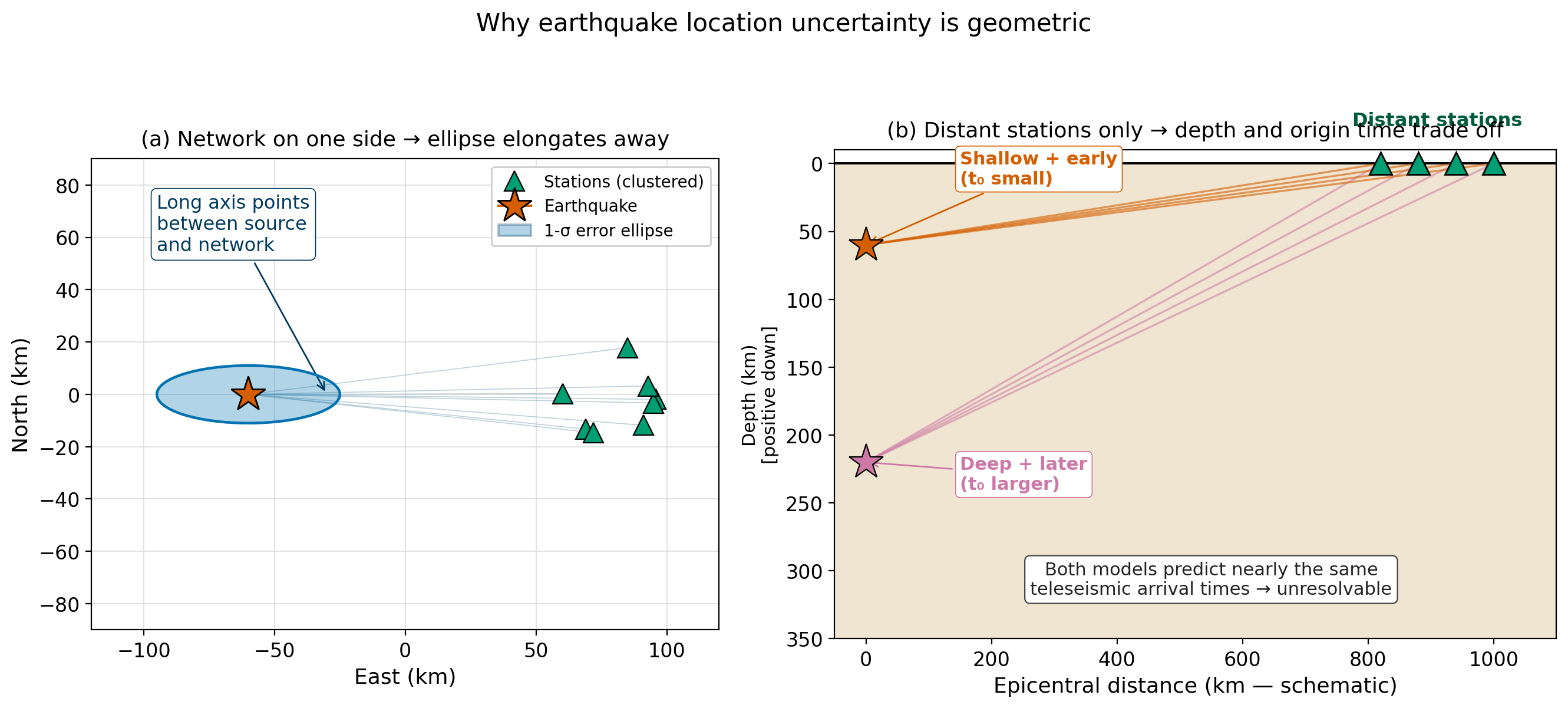— Fig. 64 The geometric origin of earthquake-location uncertainty. (a) When the recording network is clustered on one side, the error ellipse is elongated radially away from the network. (b) When only distant stations are available, focal depth and origin time trade off: a shallower-and-earlier source predicts the same arrival times as a deeper-and-later source.#

5b. Relative location: the double-difference principle#

When two earthquakes occur close together — say, on the same fault patch — the ray paths from each to a common station are nearly identical, and the difference of their arrival times at that station depends only on the difference of their hypocentral coordinates. The bulk of the velocity-model error, which would otherwise dominate the absolute location uncertainty, cancels out in the differencing. Algorithms that exploit this cancellation — most prominently the double-difference relocation algorithm HypoDD of Waldhauser and Ellsworth [2000] — routinely achieve relative location precisions of tens of metres for clustered earthquakes, even when the absolute locations are uncertain at the kilometre level. The result is the spectacular fault-aligned earthquake structures that emerge when raw catalogs are relocated, as in Hauksson et al. [2012] for southern California, Shelly et al. [2016] for Long Valley caldera, and the Quake Template Matching (QTM) catalog of Ross et al. [2019] for the San Jacinto fault zone.

6. A worked example: locating a small Puget Lowland earthquake#

A small earthquake occurs in the Puget Lowland. A three-component PNSN station, \(50\) km from the epicenter, records a clean P arrival at \(T_P = 14.2\) s and a clean S arrival at \(T_S = 21.1\) s in absolute time after some reference. The horizontal first-motion amplitudes are \(A_N = 0.74\) and \(A_E = 0.32\) on a normalized scale, with a clear upward Z first motion. Take \(V_P = 6.0\) km/s and \(V_S = 3.46\) km/s in the upper crust.

Hypocentral distance from S-minus-P. The S-minus-P time is \(T_S - T_P = 6.9\) s. From equation (109),

\[ D \;=\; \frac{6.0 \times 3.46}{6.0 - 3.46} \times 6.9 \;\approx\; 8.18 \times 6.9 \;\approx\; 56\ \mathrm{km}. \]

Back-azimuth from polarization. From equation (110),

\[ \mathrm{AZI} \;=\; \arctan(0.32 / 0.74) \;\approx\; 23.4°. \]

The upward Z first motion confirms that the ray came from below and to the NNE; the back-azimuth is therefore \(\mathrm{BAZ} \approx 23°\) — meaning the epicenter lies roughly \(23°\) east of north as seen from the station.

Concept check. The catalog shows the PNSN’s nearest dense cluster of stations is in central Puget Sound, and the epicentral distance is \(\Delta = 50\) km while the hypocentral distance is \(D = 56\) km. From equation (111), the focal depth is

\[ h \;=\; \sqrt{56^2 - 50^2} \;\approx\; 25\ \mathrm{km}. \]

A \(25\) km focal depth in this region is consistent with a deep intra-slab event in the subducting Juan de Fuca plate beneath Puget Sound — the same regime as the 2001 \(M_w\) 6.8 Nisqually earthquake.

Concept-check questions

If the analyst had used a velocity model with \(V_P = 5.5\) km/s instead of \(6.0\) km/s (and the same \(V_P/V_S\) ratio), how would the calculated hypocentral distance change?
Which of the two distance estimates — single-station \(D\) or multi-station triangulated epicenter — would you trust more for an event \(\Delta = 5\) km from the closest station? Why?
If only teleseismic stations had recorded this event, which of the four source parameters \((x_0, y_0, z_0, t_0)\) would be best constrained, and which would be most degenerate?

7. Connecting to Cascadia: ShakeAlert and societal relevance#

The Pacific Northwest’s ShakeAlert earthquake early-warning system became operational for Washington and Oregon in 2021. ShakeAlert ingests data from the PNSN’s \(\sim 1500\) seismic stations, plus geodetic data from \(\sim 760\) GNSS sensors, and uses real-time location and magnitude estimation to issue alerts seconds to tens of seconds before the strong shaking from a damaging earthquake reaches a given location. The warning time available to a user depends on (a) how rapidly the location and magnitude can be determined, and (b) how far the user is from the source.

For a Cascadia subduction-zone megathrust earthquake initiating offshore, a user in Seattle would typically receive several tens of seconds of warning; a user on the immediate coast would receive much less. For deeper intra-slab events such as the 2001 Nisqually earthquake, computer simulations indicate that ShakeAlert can typically deliver about 10 seconds of warning before strong shaking arrives at the surface. The accuracy of these warnings depends directly on how accurately and how rapidly the system performs the location problem of this lecture — a real-time inverse problem with hard latency budgets.

A complementary algorithm, GFAST (Geodetic First Approximation of Size and Time), developed by PNSN researchers at the University of Washington, uses GNSS-measured ground displacements rather than seismic-station velocities to estimate the magnitude of the largest events without saturating. Seismic magnitude estimates saturate near \(M_w\) 7 because regional stations cannot detect the long-period radiation that distinguishes a \(M_w\) 7 earthquake from a \(M_w\) 9 earthquake on the basis of peak acceleration alone; geodetic displacement scales linearly with seismic moment regardless of size and so does not saturate [Pacific Northwest Seismic Network, 2024]. The integration of GFAST into ShakeAlert, completed in 2024, is a direct application of the forward / inverse problem framework of this lecture to a different physical observable.

For students wishing to follow up: the PNSN web portal at pnsn.org publishes real-time earthquake locations, daily activity summaries, and an extensive set of educational resources including the N Yo’ Seismic Network video series. The companion lab for this week uses ObsPy to query the PNSN catalog, retrieve waveforms, and reproduce a single-station S-minus-P distance estimate from real data.

8. Research Horizon#

Two technological shifts have transformed earthquake location since roughly 2018, and both will be operational in the Pacific Northwest by the time today’s undergraduates begin graduate work.

Machine-learning phase pickers. Convolutional and transformer neural networks now pick P and S arrivals on continuous waveform data with precision approaching that of expert analysts, but at orders-of-magnitude greater throughput. PhaseNet [Zhu and Beroza, 2019], a U-Net trained on \(\sim\) 600,000 hand-picked Northern California waveforms, achieves \(\sim\) 96% precision on P-wave detection. EQTransformer [Mousavi et al., 2020] adds a hierarchical attention mechanism and outperforms all earlier pickers on a global benchmark dataset. Multi-station extensions such as the Phase Neural Operator (PhaseNO) [Sun et al., 2023] exploit the spatial coherence of arrivals across a network, and a re-trained EQTransformer applied to two decades of PNSN data has produced the first machine-learning earthquake catalog for the Pacific Northwest, with substantial gains in event completeness for small magnitudes. These methods should be understood not as replacements for the physics in section 3 but as fast, automated front-ends that supply the picks \(\{T_P^{(i)}, T_S^{(i)}\}\) that the location problem then consumes.

Distributed acoustic sensing (DAS). A single fibre-optic cable, interrogated with laser pulses from one end, can be turned into a dense seismic array of thousands of “channels” spaced metres apart along the cable. Submarine telecommunication fibres off the Cascadia margin have recently been used to detect and locate offshore earthquakes that no land-based instrument could record adequately [Wilcock et al., 2025], and the integration of DAS into earthquake early-warning systems is now active research. The Denolle group at the University of Washington has been particularly active in developing semi-supervised learning approaches for picking phases on DAS data [Zhu et al., 2023] and in evaluating the offshore early-warning gain from submarine cables.

Earthquake catalogs as research products. The combination of dense networks, ML picking, and double-difference relocation has produced a generation of “high-resolution” catalogs that resolve fault structures at metre to hundred-metre scale. Ross et al. [2019] produced the QTM catalog of \(1.81\) million events on the San Jacinto fault zone using template matching at the waveform level; Shelly et al. [2016] resolved the structure of a 2014 Long Valley caldera swarm in three dimensions with relative precision approaching \(20\) metres. These catalogs are themselves data products on which derivative research — earthquake-rate forecasting, fault-zone structural geology, induced-seismicity attribution — increasingly depends.

9. AI Literacy: when to trust an automated phase pick#

AI Epistemics — phase pickers and the data they were trained on

Modern machine-learning phase pickers are remarkably good — until they are not. The PhaseNet and EQTransformer benchmark figures cited in section 8 (precision and recall around 95% on test sets) describe performance on data that look like their training data. Independent evaluations have found that the recall of pre-trained pickers can drop by 30–40% when applied to a new region [Münchmeyer et al., 2022], and dramatically further on unusual data types — ocean-bottom seismograms, downhole data sampled at \(2000\) Hz, distributed-acoustic-sensing strain rates, or mining-induced microseismicity. A pre-trained model is a prior about what waveforms look like, and that prior fails when the new data fall outside the training distribution.

For this course’s purposes, three habits matter:

Always know the training distribution. Before using any pre-trained phase picker on real data, locate the original paper and identify (i) the geographic region, (ii) the magnitude range, (iii) the sampling rate, and (iv) the sensor type used to assemble the training set. If your target data differs in any of these dimensions, expect degraded performance.
Always verify a sample by eye. Even at 95% recall, a network with 200 candidate detections in a 24-hour record will have \(\sim 10\) false positives and miss \(\sim 10\) true events. Manual inspection of a small random sample is the only practical way to characterize what kind of mistakes the picker is making for your problem.
Always carry the velocity-model assumption forward. A phase pick is just an arrival time. The location estimate built from those picks is no better than the velocity model used in the forward operator. ML pickers do not absolve the user from understanding the velocity structure beneath the network.

Prompt Lab — interrogating an AI explanation of an earthquake catalog

Try the following prompts with an AI assistant. For each, evaluate the response against the criteria below.

Prompt 1: “Summarize, in three sentences, why machine-learning phase pickers like PhaseNet and EQTransformer increase the number of detected earthquakes in a given region.”

Prompt 2: “Why is the depth of a teleseismically recorded earthquake more uncertain than its epicenter?”

Prompt 3: “List three known failure modes of pre-trained ML phase pickers, with citations.”

Evaluation criteria:

Did the AI distinguish between detection (finding events) and picking (timing arrivals)?
Did the AI cite the depth–origin-time trade-off in geometric terms, or did it appeal to vague claims about “ray angles”?
Are the citations real? Search each title to verify it is a published paper, not a hallucinated reference.
Did the response acknowledge any of the limitations described above, or did it present ML pickers as uniformly successful?

10. Concept Checks#

Synthesis questions

Phase identification. A three-component station records, in order, a small high-frequency arrival, a larger lower-frequency arrival, and a long-period dispersive train of largest amplitude. Identify each phase and explain in one sentence each why this order is universal.
Velocity-model sensitivity. If your assumed \(V_P\) is too high by 5 % (with \(V_P/V_S\) fixed), in which direction does your single-station distance estimate err, and by approximately what percentage?
Network geometry. Sketch a station distribution that produces a circular (rather than elongated) error ellipse. Sketch one that produces an east–west–elongated ellipse.
Depth–origin-time trade-off. A \(10\) km change in focal depth at teleseismic distance is compensated by roughly what change in origin time? Why does the depth phase pP break this trade-off?
Linear vs. non-linear. Of the four source parameters \((x_0, y_0, z_0, t_0)\), which one is recovered by a single linear matrix step and which three require iteration? Why?
Relative location. Two earthquakes a few hundred metres apart can be relatively located to tens of metres even when their absolute locations are uncertain at the kilometre level. Which physical quantity cancels in the differencing?
Beyond Earth. Mars’s InSight mission used a single three-component seismometer to locate marsquakes. Which of the multi-station techniques in section 3 had to be replaced by polarization-based reasoning, and what kind of uncertainty did that introduce?

11. Connections#

The location problem is the same family of problem as the seismic-tomography problem of Lecture 12, but with a different unknown. In tomography, the velocity field is the unknown and the source-receiver geometry is fixed; in location, the velocity field is fixed (assumed) and the source position is the unknown. The forward operator \(G_i\) is a travel-time integral in both cases. Modern joint inversions — in which the source positions and the velocity model are estimated simultaneously — are routine in regional seismic networks, and they connect this lecture directly to the imaging methods of Module 3.

The forward / inverse-problem framework introduced here will reappear in Lecture 19 (Earth’s gravity) and Lecture 23 (Earth’s magnetic field), where the observable is no longer a travel time but a gravity or magnetic anomaly. The non-uniqueness identified in section 5 is a general feature of geophysical inverse problems, not a peculiarity of seismology.

The next lecture, Earthquake Phenomena II, takes the location \((x_0, y_0, z_0, t_0)\) as a known quantity and turns to the question of how big the earthquake was — magnitude scales, the seismic moment \(M_0\), and the connection to the radiated wavefield amplitude.


Course LOs addressed	LO-1, LO-2, LO-3, LO-5, LO-7
Learning outcomes practiced	LO-OUT-A (sketch geometry), LO-OUT-B (compute travel times), LO-OUT-D (set up inverse problem), LO-OUT-E (interpret residuals and non-uniqueness), LO-OUT-H (critique AI-generated catalogs)
Prior lecture	Lecture 12 — Seismic Tomography: introduces the forward/inverse problem in a pure imaging context
Next lecture	Lecture 14 — Earthquake Phenomena II: magnitude, source spectra, and focal mechanisms
Lab connection	Lab on phase picking and earthquake location with `ObsPy` (week 5)