Earthquake Phenomena II — Magnitude, Energy, and Statistics

Earthquake Phenomena II — Magnitude, Energy, and Statistics#

Prerequisites#

Students should be comfortable with: base-ten logarithms and the power-of-ten interpretation of an order of magnitude (the slide-set review on the first lecture day is sufficient); the elastic shear modulus and Hooke’s law (Lecture 3); P-, S-, and surface-wave phases on a seismogram (Lectures 4 and 5); and the meaning of fault area, slip, and rigidity (Lecture 13).

1. The framing question: how do we put a single number on an earthquake?#

On 11 March 2011, the Tōhoku-oki megathrust ruptured a 500 km × 200 km patch of the Japan Trench. Average slip exceeded 25 m. The P-wave arrived at the PNSN station NEW in eastern Washington 12 minutes later, with a peak vertical displacement of about 0.6 mm — three hundred times the displacement that the same station records during the typical Pacific Northwest microearthquake. By the time the surface waves swept through, NEW had moved through several centimetres. Within an hour, every seismological agency in the world had assigned the event a single number: \(M_W\) 9.1.

That number is doing an enormous amount of work. It is meant to convey, in one quantity, the size of a rupture that lasted 150 seconds, broke a fault four times the area of the Olympic Peninsula, and released as much energy as the Earth’s entire annual seismic budget for an average year. It is meant to be comparable to the magnitude assigned to a microearthquake on the South Whidbey Island fault in 2024, recorded on the same instrument 200 km from the source. It is meant to feed directly into a tsunami-warning algorithm, a building-code update, and a paleoseismic recurrence model.

A single number cannot do all of this faithfully. The story of earthquake magnitude is the story of how seismologists have tried, since 1935, to compress a high-dimensional rupture process into a scalar — and the story of why several different scalars are needed to cover the full range of earthquake size.

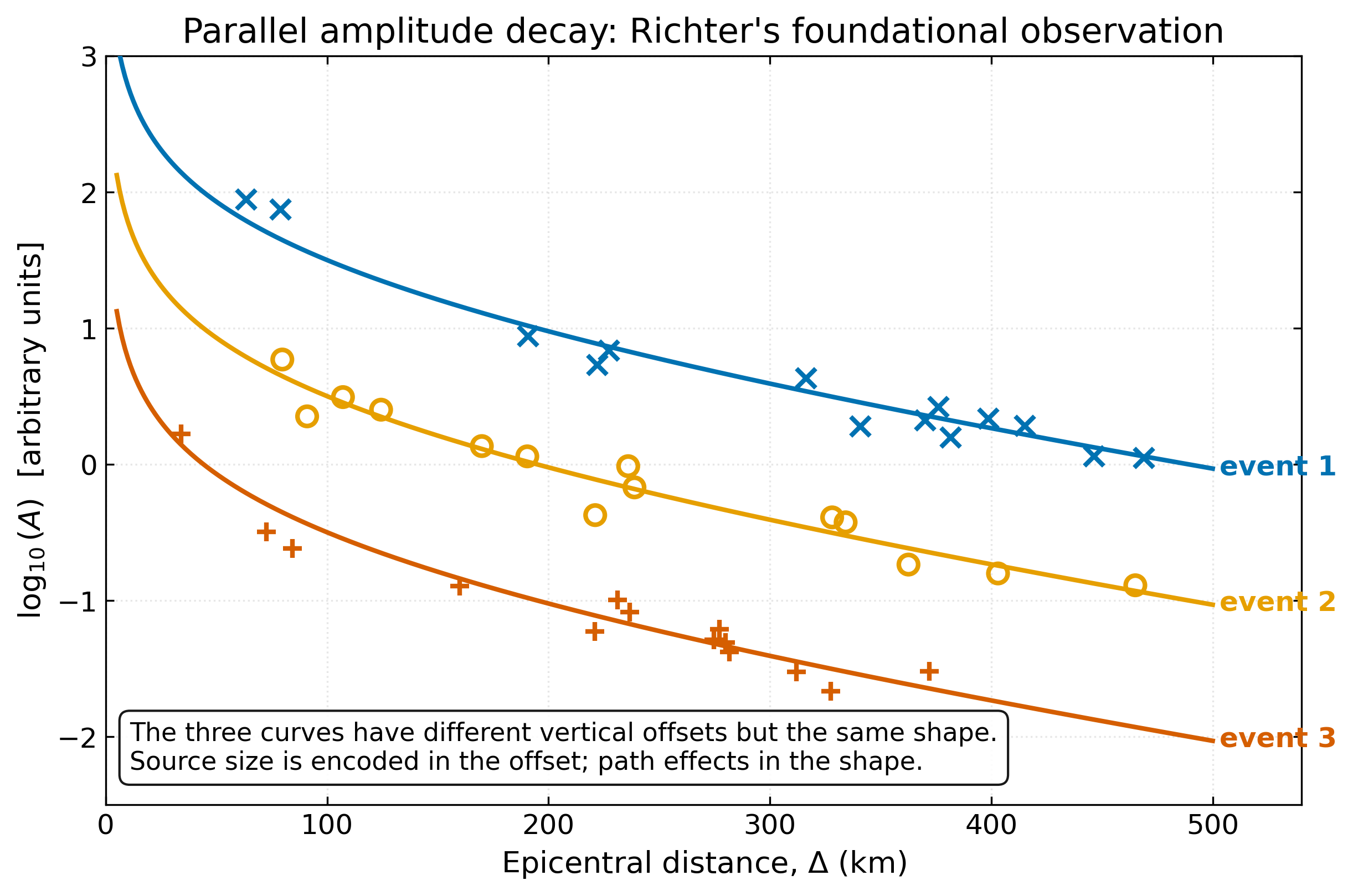
Plot of base-ten logarithm of seismic-wave peak amplitude on — Fig. 65 the vertical axis versus epicentral distance on the horizontal axis, for three hypothetical earthquakes labeled event 1, event 2, and event 3. Three curves descend smoothly from upper left to lower right; the curves are parallel within scatter, separated by constant vertical offsets, with event 1 highest, event 2 in the middle, and event 3 lowest. Markers (crosses for event 1, circles for event 2, plus signs for event 3) cluster along each curve. The vertical offset between adjacent curves is approximately one unit on the log-amplitude axis. :width: 80%#

Charles Richter’s 1935 observation, the foundation of every magnitude scale used since: peak seismic-wave amplitudes from different earthquakes decay with distance along *parallel* curves on a log-amplitude vs distance plot. The shape of the curve depends on geometric spreading and attenuation in the crust; the *vertical offset* between curves depends only on the source. Therefore the offset, evaluated at a reference distance, is a stable measure of relative earthquake size. Reproduces the scientific content of Stein & Wysession (2003) Fig 9.23 from a synthetic two-parameter spreading model.

This lecture proceeds in three stages. First, we follow Richter’s historical reasoning to its modern form: the local magnitude \(M_L\), and the body- and surface-wave magnitudes \(m_b\) and \(M_S\) that extended it to teleseismic distances (§2-3). Second, we develop the seismic moment \(M_0\) — a physical measure of fault slip — and the moment magnitude \(M_W\) that is calibrated to it (§4-5). Third, we turn from individual events to populations of earthquakes: the Gutenberg-Richter frequency-magnitude law and the Omori aftershock law (§6). Throughout, the Pacific Northwest serves as the running example, because the Cascadia subduction zone produces the full spectrum from \(M_L\) -1 swarms to the \(M_W\) 9 paleoseismic events recorded in turbidite sequences off the Oregon coast.

2. The physics: why a logarithm, and why amplitudes decay with distance#

Two physical observations underlie every magnitude scale. The first is the enormous dynamic range of seismic ground motion. A microearthquake recorded at a station 5 km away might displace the ground by 1 nanometre; a great earthquake at the same station can displace it by 10 metres. The ratio is \(10^{10}\). No linear scale can usefully present this range to a human reader, just as no linear scale is used for sound (decibels), star brightness (magnitudes), or acidity (pH). The base-ten logarithm compresses ten orders of magnitude into a span of ten units.

Important

Key concept: the logarithmic compression of magnitude

Each whole-number step on a magnitude scale corresponds to a factor of ten in seismic-wave amplitude. The ratio of physical quantities is recovered by exponentiation:

Magnitude difference	Amplitude ratio	Approximate energy ratio
1 unit	\(10^1 = 10\)	\(\sim 32\)
2 units	\(10^2 = 100\)	\(\sim 1\,000\)
3 units	\(10^3 = 1\,000\)	\(\sim 32\,000\)

The energy ratio is the amplitude ratio raised to the power \(3/2\), because radiated seismic energy scales as the integral of velocity squared over the duration of the rupture, and rupture duration also grows with size (§4). One magnitude unit therefore corresponds to roughly \(10^{1.5} \approx 31.6\) times the radiated energy.

The second observation is that seismic-wave amplitudes attenuate with distance from the source. A wave radiating spherically from a point source spreads its energy over a surface area that grows as \(4\pi r^2\), so the energy per unit area decreases as \(1/r^2\) and the displacement amplitude as \(1/r\) — geometric spreading. In addition, real rocks dissipate elastic energy into heat, so amplitude is further reduced by a factor that decays roughly exponentially with travel distance — anelastic attenuation. Both processes mean that two stations recording the same earthquake see different amplitudes; the deeper one or the more distant one sees less.

Richter’s empirical insight in 1935 was that the shape of the amplitude-distance decay curve is approximately the same for every local earthquake — it is a property of the medium, not the source — while the vertical offset between curves depends only on the source. This is the content of Fig. 65. If we read off the amplitude at a fixed reference distance, we eliminate the path effect and isolate a number that scales with rupture size.

3. Mathematical framework: a hierarchy of magnitudes#

Notation

Symbol	Meaning	Units
\(A\)	Peak ground-motion amplitude on a seismogram	mm or μm
\(T\)	Period of the wave at which \(A\) is measured	s
\(\Delta\)	Epicentral distance, or angular distance for teleseisms	km or degrees
\(h\)	Source depth	km
\(M_L\)	Local (Richter) magnitude	dimensionless
\(m_b\)	Body-wave magnitude (P-wave)	dimensionless
\(M_S\)	Surface-wave magnitude (Rayleigh wave at \(T = 20\) s)	dimensionless
\(M_0\)	Scalar seismic moment	N·m
\(M_W\)	Moment magnitude	dimensionless
\(\mu\)	Shear modulus (rigidity) of fault-zone rock	Pa
\(A_f\)	Fault area	m²
\(\bar{s}\)	Average slip on the fault	m
\(E_S\)	Radiated seismic energy	J

3a. Local magnitude \(M_L\) — Richter’s original scale#

Richter (1935) defined the local magnitude as

(117)#\[ M_L \;=\; \log_{10}(A) \;-\; \log_{10}(A_0(\Delta)), \]

where \(A\) is the maximum trace amplitude in millimetres on a standard Wood-Anderson torsion seismograph (a specific instrument with a natural period of 0.8 s and magnification of 2800), and \(A_0(\Delta)\) is an empirically tabulated reference amplitude that absorbs all distance and path effects. By construction, \(M_L = 3\) when \(A = 1\) mm at \(\Delta = 100\) km on the Southern California crust. The distance correction \(-\log_{10} A_0(\Delta)\) is what Fig. 66 shows.

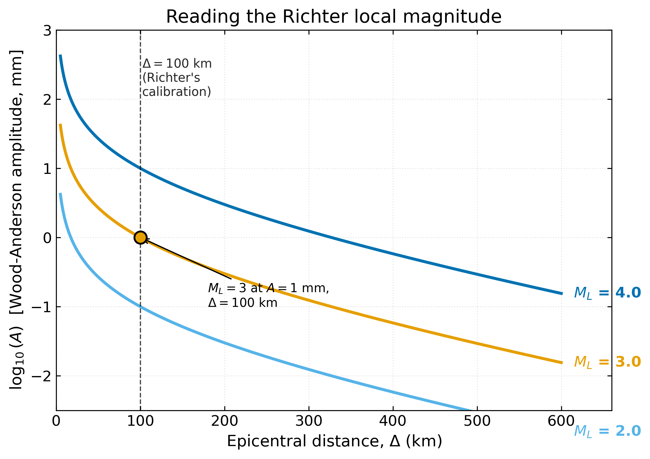
Plot of base-ten logarithm of peak seismogram amplitude on — Fig. 66 the vertical axis versus epicentral distance on the horizontal axis. Three smooth curves slope downward from upper left to lower right, labeled at the right edge with local magnitude values M_L equal to 4.0 (highest curve, blue), M_L equal to 3.0 (middle curve, orange), and M_L equal to 2.0 (lowest curve, sky blue). The curves are equally spaced vertically by one unit, reflecting the one-magnitude-equals-tenfold-amplitude rule. A dashed vertical reference line at distance equals 100 kilometres marks Richter’s calibration distance. :width: 70%#

The Richter nomogram. Reading \(M_L\) from a station record requires two numbers: the peak Wood-Anderson amplitude \(A\) and the epicentral distance \(\Delta\) (estimated from the S-P time). The distance correction \(-\log_{10} A_0(\Delta)\) accounts for geometric spreading and crustal attenuation. The same source produces three different \(\log A\) readings at three different distances, but all three give the same \(M_L\) once the correction is applied.

In modern practice, \(M_L\) is no longer measured on Wood-Anderson seismographs — there are essentially none left in routine operation — but on broadband instruments whose ground-motion records are synthesised into the response of a virtual Wood-Anderson, so that the resulting \(M_L\) can be compared to the historical catalogue.

3b. Body-wave magnitude \(m_b\) and surface-wave magnitude \(M_S\) — extending the scale globally#

The Wood-Anderson seismograph saturates above \(\Delta \approx 600\) km because the highest-frequency content of the wavefield (which the instrument is sensitive to) dies off rapidly with distance. Two generalisations were introduced to handle teleseismic earthquakes recorded at hundreds or thousands of kilometres:

Key equations: teleseismic body- and surface-wave magnitudes

(118)#\[ m_b \;=\; \log_{10}\!\!\left(\frac{A}{T}\right) \;+\; Q(\Delta, h) \]

(119)#\[ M_S \;=\; \log_{10}\!\!\left(\frac{A}{T}\right) \;+\; 1.66\,\log_{10}(\Delta) \;+\; 3.30 \]

For \(m_b\), \(A\) is the peak P-wave displacement (in μm) measured at about 1 s period on a short-period instrument; \(Q(\Delta, h)\) is a tabulated path correction that depends on epicentral distance and source depth. For \(M_S\), \(A\) is the peak Rayleigh-wave displacement measured at \(T = 20\) s on a long-period instrument; the explicit distance term replaces a tabulated \(Q\) because long-period surface waves attenuate predictably along the great-circle path.

Equations (118) and (119) are designed to agree with \(M_L\) in the magnitude range 4-6 where they overlap. The point of the overlap is to maintain a single magnitude history across instrument generations and event sizes. Earthquakes with \(M_L < 3\) are too small to register at teleseismic distances and have only \(M_L\); earthquakes with \(M > 7\) are too big to be recorded without clipping at local distances and have only \(m_b\) and \(M_S\).

3c. The saturation problem#

A subtle defect haunts the wave-amplitude magnitudes \(M_L\), \(m_b\), and \(M_S\): each is measured at a fixed period — about 0.1 s for \(M_L\), 1 s for \(m_b\), 20 s for \(M_S\). For a small earthquake the rupture lasts a fraction of a second and the radiated wavefield has plenty of energy at all three of those periods. For a great earthquake the rupture lasts a minute or more and most of the radiated energy is at periods far longer than 20 s. The peak amplitude at 1 s (\(m_b\)) and at 20 s (\(M_S\)) becomes insensitive to further increases in rupture size — the magnitude saturates. Fig. 67 makes this explicit:

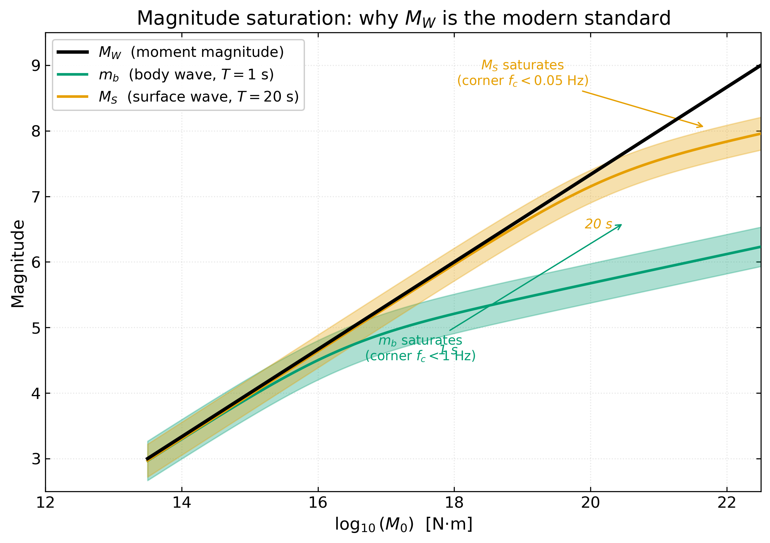
Plot of magnitude on the vertical axis versus seismic moment — Fig. 67 in newton-metres on the horizontal axis, with the moment axis on a base-ten logarithmic scale running from ten to the twelfth to ten to the twenty-second. A solid black line labeled M_W rises linearly across the entire plot, reaching magnitude 9 at moment ten to the twenty-second. A grey corridor labeled m_b follows M_W up to about magnitude 6.5 and then bends over and flattens at magnitude 6 to 7 for higher moments. A second grey corridor labeled M_S follows M_W up to about magnitude 8.0 and then bends over and flattens near magnitude 8 to 8.3. Two dashed lines labeled twenty seconds and one second show theoretical predictions for an omega-squared source spectrum at those two periods, matching the M_S and m_b corridors respectively. :width: 80%#

Magnitude saturation. The moment magnitude \(M_W\) (solid line) tracks seismic moment \(M_0\) over the entire range. The body-wave magnitude \(m_b\) (1-s period) saturates near 6-7; the surface-wave magnitude \(M_S\) (20-s period) saturates near 8-8.3. The dashed lines are the predictions of the Madariaga (1976) circular crack source model with stress drop 3 MPa, evaluated at 1 s and 20 s. The saturation is not a measurement artefact — it is a consequence of measuring the radiated wavefield at a fixed period for a source whose characteristic period grows with size. Reproduces the scientific content of Stein & Wysession (2003) Fig 9.25.

3d. Seismic moment \(M_0\) and moment magnitude \(M_W\)#

The cleanest way out of the saturation problem is to measure something that is not tied to a fixed period. The seismic moment provides exactly that. For a fault of area \(A_f\) that has slipped on average by \(\bar{s}\), in a medium of shear modulus \(\mu\),

Key equation: scalar seismic moment

(120)#\[ M_0 \;=\; \mu \, A_f \, \bar{s} \]

Units: \(M_0\) is reported in newton-metres (N·m). The historical literature also uses dyne-centimetres (dyne·cm), with \(1\;\text{N·m} = 10^7\;\text{dyne·cm}\). Crustal rigidity is typically \(\mu \approx 30\;\text{GPa}\) for shallow continental rock and rises to \(\mu \approx 70\;\text{GPa}\) in the deep upper mantle.

Equation (120) is purely geometric and mechanical: it does not care what period we measure at. It can be obtained from low-frequency seismic-wave inversion, from geodetic measurements of static displacement (GPS, InSAR), or directly from field measurements of slip on the surface trace of a fault.

Hanks & Kanamori (1979) defined the moment magnitude \(M_W\) as a linear function of \(\log_{10} M_0\) chosen to match \(M_S\) in the range where \(M_S\) is reliable:

Key equation: moment magnitude

(121)#\[ M_W \;=\; \tfrac{2}{3}\,\log_{10}(M_0) \;-\; 6.03 \quad \text{(SI units, } M_0 \text{ in N·m)} \]

Equivalently, \(\log_{10} M_0 = 1.5\,M_W + 9.0\). The factor of \(2/3\) is not arbitrary — it follows from the proportionality between radiated seismic energy \(E_S\) and \(M_0\) in a self-similar source model (Kanamori, 1977).

Because \(M_0\) does not saturate, neither does \(M_W\). For ordinary earthquakes (\(M_W \lesssim 7\)), all of \(M_L\), \(m_b\), \(M_S\) and \(M_W\) agree to within a few tenths of a unit. For great earthquakes (\(M_W \gtrsim 8\)), only \(M_W\) remains a reliable measure of true size. The “9.1” assigned to Tōhoku is a moment magnitude.

4. The forward problem: predicting an earthquake’s magnitude from its physics#

Given a description of a fault — its dimensions, its average slip, the rigidity of the rock around it — equation (120) directly predicts the seismic moment, and equation (121) then converts \(M_0\) to \(M_W\). This is the forward problem of earthquake size: from a model of the rupture, predict the observable.

Worked example: the moment of a “garden-variety” \(M_W \approx 6\) earthquake

Take a square fault patch 10 km on a side, slipping on average by 1 m, in continental crust of rigidity \(\mu = 30\) GPa.

\[\begin{align*} A_f &= 10\;\text{km} \times 10\;\text{km} = 10^4 \times 10^6 \;\text{m}^2 = 10^{10}\;\text{m}^2 \\ \bar{s} &= 1\;\text{m} \\ \mu &= 3 \times 10^{10}\;\text{Pa} \\ M_0 &= \mu A_f \bar{s} = (3\times 10^{10})(10^{10})(1) = 3 \times 10^{20}\;\text{N·m} \end{align*}\]

Wait — that gives \(M_W = (2/3)\log_{10}(3\times 10^{20}) - 6.03 \approx 7.6\), not 6. The trick is that 10 km × 10 km is much too large for a magnitude-6 fault: real \(M_W\) 6 events typically rupture patches 3-5 km on a side with about 0.1-0.3 m of average slip. Plug those in: \(A_f \approx 10^7\;\text{m}^2\), \(\bar{s} \approx 0.2\;\text{m}\), \(M_0 \approx 6 \times 10^{16}\;\text{N·m}\), and \(M_W \approx 5.1\). The qualitative lesson: rupture area and slip both grow with magnitude, by roughly self-similar scaling, so a 10× increase in linear fault dimension and a 10× increase in slip produce a \(10 \times 10 \times 10 = 1000\times\) increase in moment, which is two units of magnitude.

The same logic can be inverted to ask how a fault must look to produce a given magnitude — the basis of the scaling questions on slide 13 of the original deck:

Concept check: magnitude-area scaling

(a) A shallow \(M_W\) 7 ruptures with \(\bar{s} = 10\) m in crust of rigidity \(\mu = 10^{10}\) Pa. A deep \(M_W\) 7 (e.g. an intermediate- depth slab event) ruptures with the same \(\bar{s} = 10\) m but in material with \(\mu = 10^{11}\) Pa. By what factor do their fault areas differ? By what factor do the radii of equivalent circular ruptures differ?

Hint: \(M_0\) is the same for both (same \(M_W\)). From \(M_0 = \mu A_f \bar{s}\), the ratio \(A_{f,\text{deep}} / A_{f,\text{shallow}} = \mu_{\text{shallow}}/\mu_{\text{deep}} = 1/10\). The deep event needs only one tenth the area for the same moment, because the rock is ten times stiffer. For circular ruptures of radius \(r\), \(A_f = \pi r^2\), so the radius ratio is \(\sqrt{1/10} \approx 0.32\).

(b) A shallow \(M_W\) 6 ruptures in the same material as the shallow \(M_W\) 7 above, with the same \(\bar{s} = 10\) m. By what factor are its fault area and radius smaller? (Answer: area ratio is \(10^{-1.5} \approx 0.032\); radius ratio is \(\sqrt{0.032} \approx 0.18\). Note that 10 m of slip on a magnitude-6 fault is unphysically large — real \(M_W\) 6 events have \(\bar{s}\) of order 0.1-0.3 m. The thought experiment isolates the moment scaling.)

5. The inverse problem: estimating \(M_0\) from seismograms#

The other direction — from observed waveforms to seismic moment — is the inverse problem. In its simplest form, the long-period spectrum of the radiated seismic wavefield approaches a constant as period grows long, and that constant is directly proportional to \(M_0\). In practice, modern seismological agencies do this in three increasingly sophisticated ways:

Long-period amplitude proxies. Reported within seconds of an earthquake, e.g. the Goldberg et al. (2024) peak-ground-displacement (\(P_d\)) estimator used in the USGS ShakeAlert system. These give a rapid magnitude with \(\sim 0.3\) unit uncertainty.
Centroid moment tensor (CMT) inversion. The fully fledged solution, fitting low-frequency body and surface waves to a point moment-tensor source. Reported within tens of minutes by the GCMT project and the USGS NEIC. Uncertainty ~0.1 unit.
Finite-fault inversion. The richest inversion, mapping slip on a discretised fault plane. Yields \(A_f\), \(\bar{s}(x,y)\), and the rupture history — but is computationally expensive and typically published days after the event.

All three are inverse problems in the formal sense of Lectures 10 and 12: a forward operator (the elastodynamic response of the Earth, truncated to long periods) maps a model parameter (the moment) to data (a waveform), and the data are inverted with appropriate regularisation. The non-uniqueness of finite-fault inversion is particularly acute and is the subject of ongoing research.

6. From individual events to populations: Gutenberg–Richter and Omori#

The discussion so far has treated each earthquake as an isolated event. Two empirical laws govern the statistics of earthquakes viewed as a population, and both are essential for hazard assessment.

6a. The Gutenberg–Richter frequency–magnitude relation#

In a 1944 BSSA paper based on Caltech’s southern California catalogue from 1934 to 1943, Gutenberg & Richter observed that the cumulative number \(N\) of earthquakes per year exceeding magnitude \(M\) in a given region follows the power law

Key equation: the Gutenberg-Richter law

(122)#\[ \log_{10}\!\big(N(M' > M)\big) \;=\; a \;-\; b\,M \]

The intercept \(a\) measures the overall seismicity rate of the region; the slope \(b\) measures the relative proportion of large to small events. For most tectonically active regions, \(b \approx 1\), meaning that the number of \(M \geq 5\) earthquakes is about ten times that of \(M \geq 6\), which is about ten times that of \(M \geq 7\), and so on.

A \(b\)-value above 1 indicates a population unusually rich in small events relative to large (often seen in volcanic swarms and geothermal areas); a \(b\)-value below 1 indicates an unusually high proportion of large events (sometimes observed at high-stress asperities late in the seismic cycle). Departures from \(b = 1\) are modest in magnitude — typically \(b = 0.7\) to \(1.3\) — but they are operationally important because the hazard from large earthquakes is dominated by the tail of the distribution.

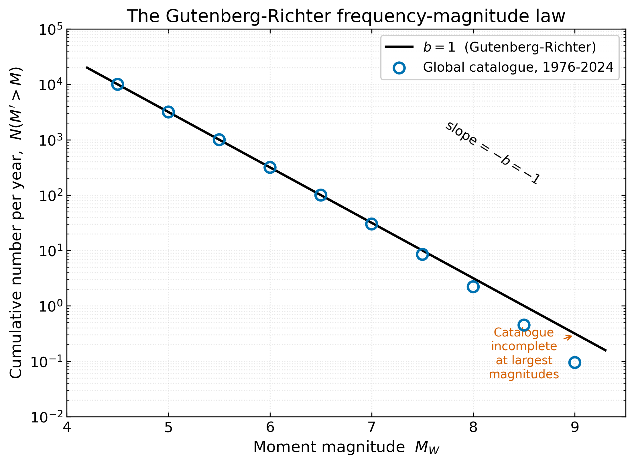
Plot of the cumulative number of earthquakes per year on the — Fig. 68 vertical axis (logarithmic, ranging from 1 to 100,000) versus moment magnitude M_W on the horizontal axis (linear, from 4 to 9). Open circles show binned earthquake counts from a global catalogue. A solid straight line through the points has slope minus one, labelled b equals 1, indicating a power-law frequency-magnitude relation. The line passes through approximately 10,000 earthquakes per year at M_W 5 and 1 earthquake per year at M_W 9. Counts at the largest magnitudes fall slightly below the line, reflecting the rarity of the largest events in the catalogue’s time window. :width: 75%#

The Gutenberg-Richter law for the global catalogue. The slope \(b \approx 1\) is the universal long-term value for most regions; the intercept \(a\) varies by region and time window. The roll-off at the largest magnitudes is partly statistical (rarity) and partly physical (no fault is large enough to host an arbitrarily large event). Reproduces the scientific content of Stein & Wysession (2003) Fig 9.27.

6b. Aftershocks and Omori’s law#

Most large earthquakes are followed by an aftershock sequence — a swarm of smaller events on or near the rupture plane, decaying with time. Two empirical regularities govern these sequences:

Båth’s law. The largest aftershock is typically about one magnitude unit smaller than the mainshock. An \(M_W\) 8 mainshock typically produces a single \(M_W \sim 7\) aftershock, ten \(M_W \sim 6\) aftershocks, a hundred \(M_W \sim 5\) aftershocks, and so on — the aftershock catalogue itself obeys a Gutenberg-Richter distribution with an intercept set by the mainshock size.
Omori’s law. The rate of aftershocks decays as a power law in time after the mainshock:

(123)#\[ n(t) \;=\; \frac{K}{(t + c)^{p}}, \qquad p \approx 1 \]

where \(K\) depends on the mainshock size, \(c\) is a small offset preventing divergence at \(t = 0\), and the exponent \(p\) is consistently close to 1 across tectonic settings.

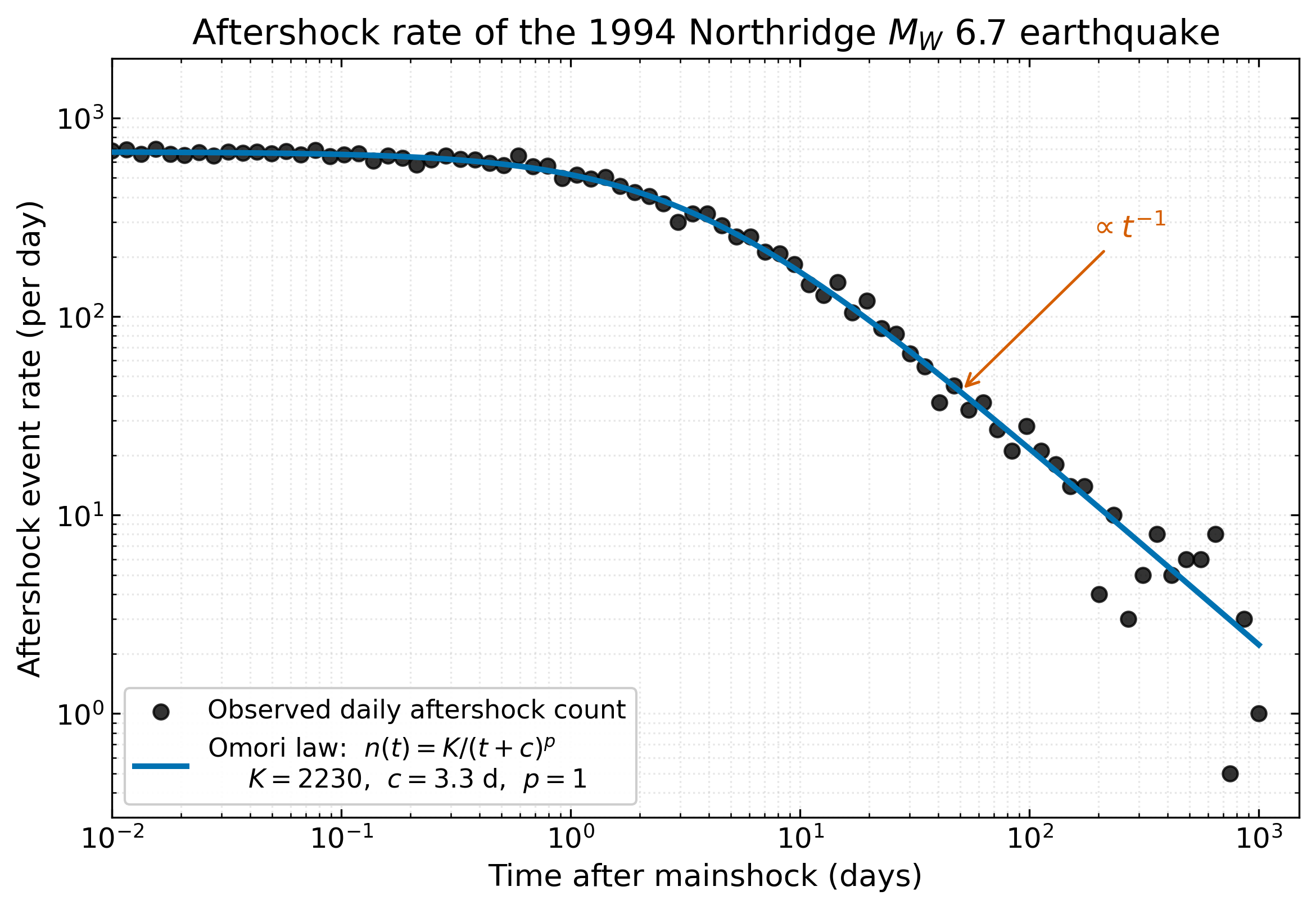
Plot of aftershock event rate per day on the vertical axis — Fig. 69 (logarithmic) versus time after the mainshock in days on the horizontal axis (logarithmic), spanning 0.01 to 1000 days. Filled circles show the observed daily aftershock rate for a real aftershock sequence. A solid black line shows the Omori-law fit with K equals 2230, c equals 3.3 days, and p equals 1. The data follow an approximately flat trend out to about one day, then decline as a power law with a slope close to minus one out to a thousand days, parallel to the labelled t-to-the-minus-one reference line. :width: 75%#

Aftershock rate of the 1994 Northridge, California \(M_W\) 6.7 earthquake, plotted on log-log axes. The data follow Omori’s law \(n(t) = K/(t+c)^p\) with \(p \approx 1\). The plateau at the earliest times reflects detection incompleteness (small aftershocks are masked by the mainshock coda) plus the small offset \(c\).

The pair of laws — Gutenberg-Richter for the size distribution, Omori for the time decay — feeds directly into operational short-term earthquake forecasting. The USGS Aftershock Forecast that appears on the event page within hours of any mainshock is a real-time evaluation of equations (122) and (123) calibrated to the mainshock magnitude.

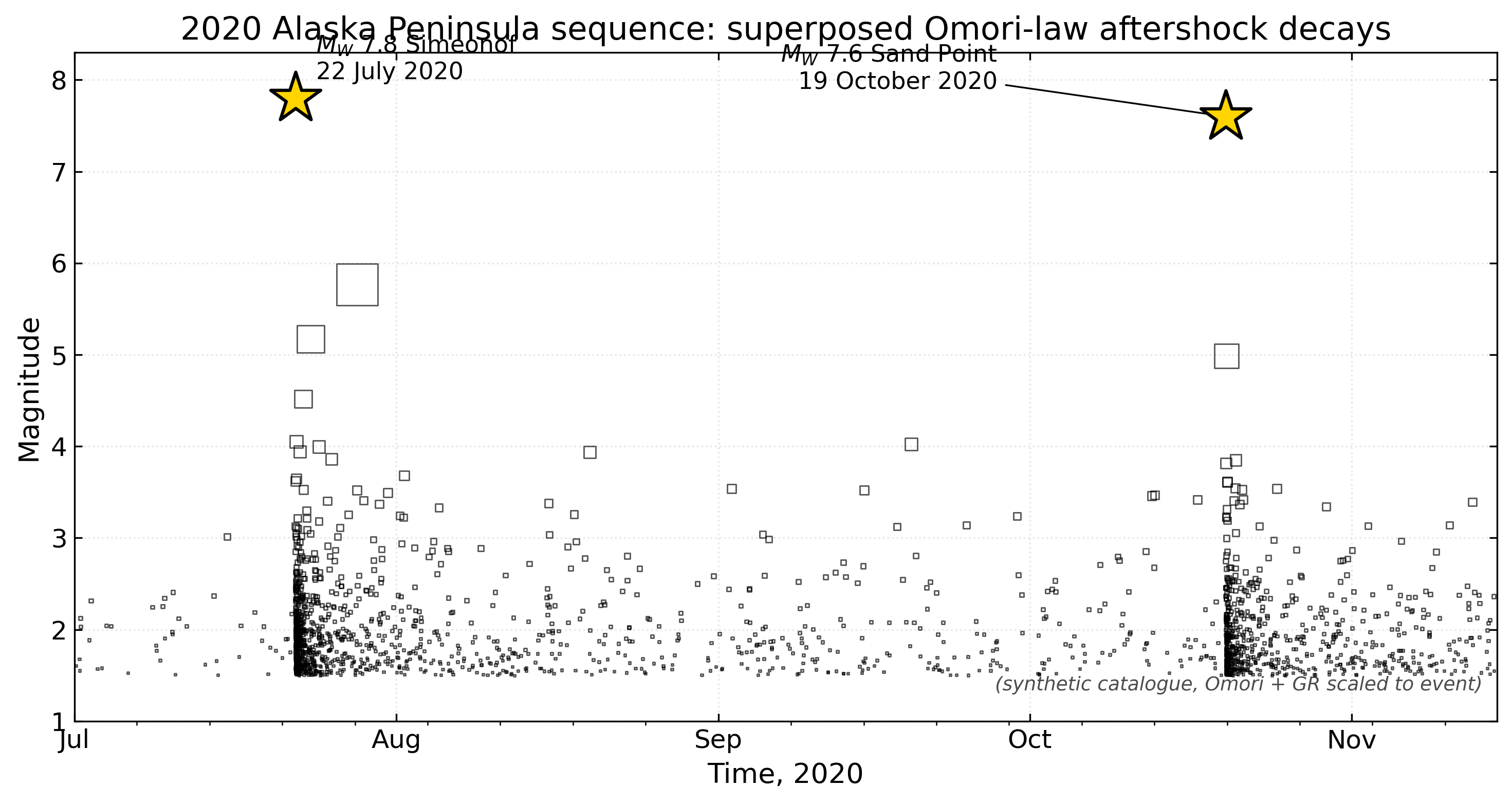
Plot of earthquake magnitude on the vertical axis versus time — Fig. 70 on the horizontal axis from July 2020 to November 2020. Each earthquake is marked by an open square; symbol size and outline width scale with magnitude. Two yellow stars mark the M7.8 mainshock on 22 July 2020 and a M7.6 doublet event on 19 October 2020. After the M7.8 mainshock, a dense cluster of aftershocks populates the plot at magnitudes from 2 to 6, with rate visibly decreasing through August, September, and October — illustrating Omori-law decay. After the M7.6 event, a second cluster of aftershocks appears, partly overlapping the decaying first sequence, illustrating that aftershock sequences superpose. :width: 90%#

Magnitude-time view of the 2020 Alaska Peninsula sequence. The \(M_W\) 7.8 Simeonof event of 22 July 2020 was followed by an Omori- law aftershock sequence; on 19 October 2020 the \(M_W\) 7.6 Sand Point event ruptured an adjacent patch of the megathrust, producing its own aftershock cluster on top of the decaying first one. Real aftershock decays are rarely “clean” — a rupture commonly triggers neighbouring ruptures days to years later. Data: USGS NEIC catalogue.

7. Connecting to Cascadia: why magnitude matters in the Pacific Northwest#

Cascadia is the place to see why every distinction in this lecture matters operationally. The subduction zone offshore of British Columbia, Washington, Oregon, and northern California has produced \(M_W \approx 9\) earthquakes on a recurrence interval of roughly 500 years, with the most recent on 26 January 1700 — established from Japanese tsunami records and from Indigenous oral histories [Atwater et al., 2005, Goldfinger et al., 2012].

For the next Cascadia event, four magnitude scales return four different numbers within the first hour after the rupture begins:

The first \(M_L\), computed from PNSN broadband stations within one S-P time of the source, is likely to read in the high 7s — a saturated value reflecting only the high-frequency content of the rupture’s first 30 seconds.
The first \(m_b\) from teleseismic stations gives a similar reading of about 7, also saturated.
The first \(M_S\) from 20-second Rayleigh waves, available within about 20 minutes, reads near 8.5.
The first \(M_W\) from a CMT-style inversion, reported within 30–60 minutes, finally returns the true value near 9.

Tsunami-warning algorithms keyed to the wrong magnitude make fundamentally different decisions. The 2011 Tōhoku event was initially assigned \(M_W\) 7.9 by JMA, then 8.4, then 8.8, and finally 9.1 — a progression that affected the timeliness and content of tsunami warnings issued to coastal Japan and the entire Pacific. Frankel et al. [2018] used 3-D wave-propagation simulations to project ground motions for hypothetical \(M_W\) 9 Cascadia earthquakes, including the strong basin amplification expected in the Seattle, Tacoma, and Portland sedimentary basins. Their results inform the current ASCE 7-22 building-code revisions and the regional earthquake early-warning thresholds.

For the deep intra-slab events such as the 2001 Nisqually \(M_W\) 6.8 earthquake — the largest Pacific Northwest event in living memory — magnitude saturation is not a concern: the rupture is short enough that \(M_L\), \(m_b\), \(M_S\), and \(M_W\) all agree to within a few tenths of a unit. Many of you may have stories from family or community about that morning of 28 February 2001; those stories are the human side of the magnitude number.

For the Pacific Northwest, the operational distinction between saturating wave-amplitude magnitudes and the non-saturating moment magnitude is not academic. It is the difference between a tsunami- warning siren that sounds and one that does not.

8. The big picture: how big are earthquakes, and how often?#

Two integrative pictures close the loop on earthquake size.

The first (Fig. 71) is the Christmas tree of earthquake energy: the relationship between magnitude, annual worldwide frequency, and equivalent chemical-explosive energy. It makes vivid the asymmetry of seismic-moment release.

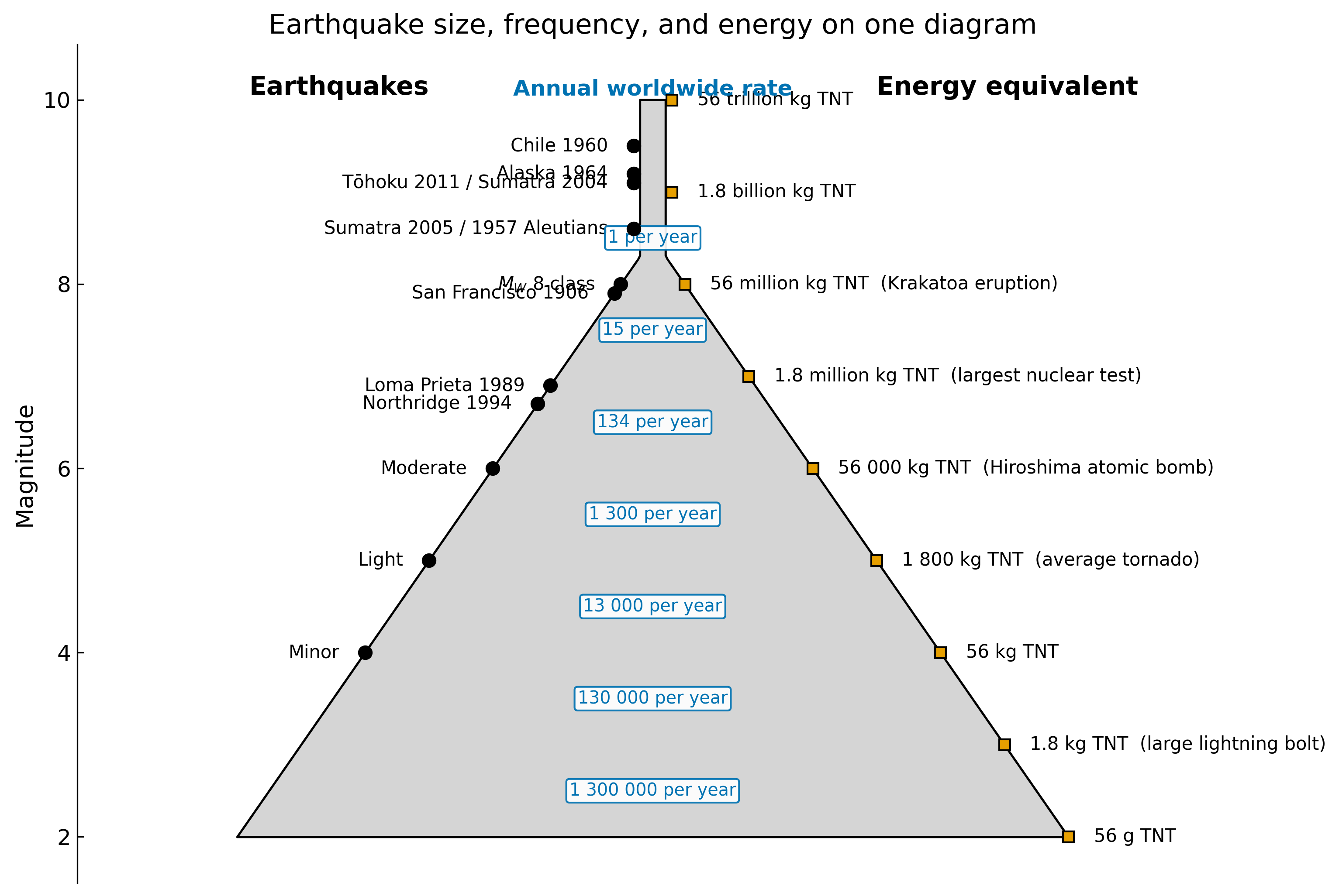
A symmetric tree-shaped figure with magnitude on the vertical — Fig. 71 axis from 2 to 10 and a horizontal width that grows from top to bottom. The left half of the tree lists earthquakes at the appropriate magnitude: Chile 1960 at 9.5 near the top, Alaska 1964 at 9.2, Tohoku 2011 at 9.1, San Francisco 1906 and Loma Prieta 1989 in the magnitude 7 range, Northridge 1994 in the high 6s, and so on. The right half labels equivalent kilograms of explosive energy, ranging from 56 trillion at magnitude 10 to about 56 thousand at magnitude 4. A horizontal axis at the bottom of the tree shows the annual worldwide number of events: about one M8 or greater per year, fifteen in the M7 range, 134 in the M6 range, and so on, growing exponentially toward smaller magnitudes. :width: 90%#

Earthquake size, frequency, and energy on a single diagram. The magnitude scale on the left is shared with the energy axis on the right, so each magnitude unit corresponds to a factor of about 32 in energy. Annual worldwide rates (centre of figure) follow the Gutenberg-Richter distribution with \(b \approx 1\). The *cumulative* moment release is dominated by the largest events: the four great earthquakes since 1900 (\(M \geq 9\)) account for nearly half of all seismic moment released in 110 years.

The second (Fig. 72) is the cumulative seismic moment record over the past 120 years, showing that the rate of moment release is set by the largest few earthquakes — not by the much more numerous small ones.

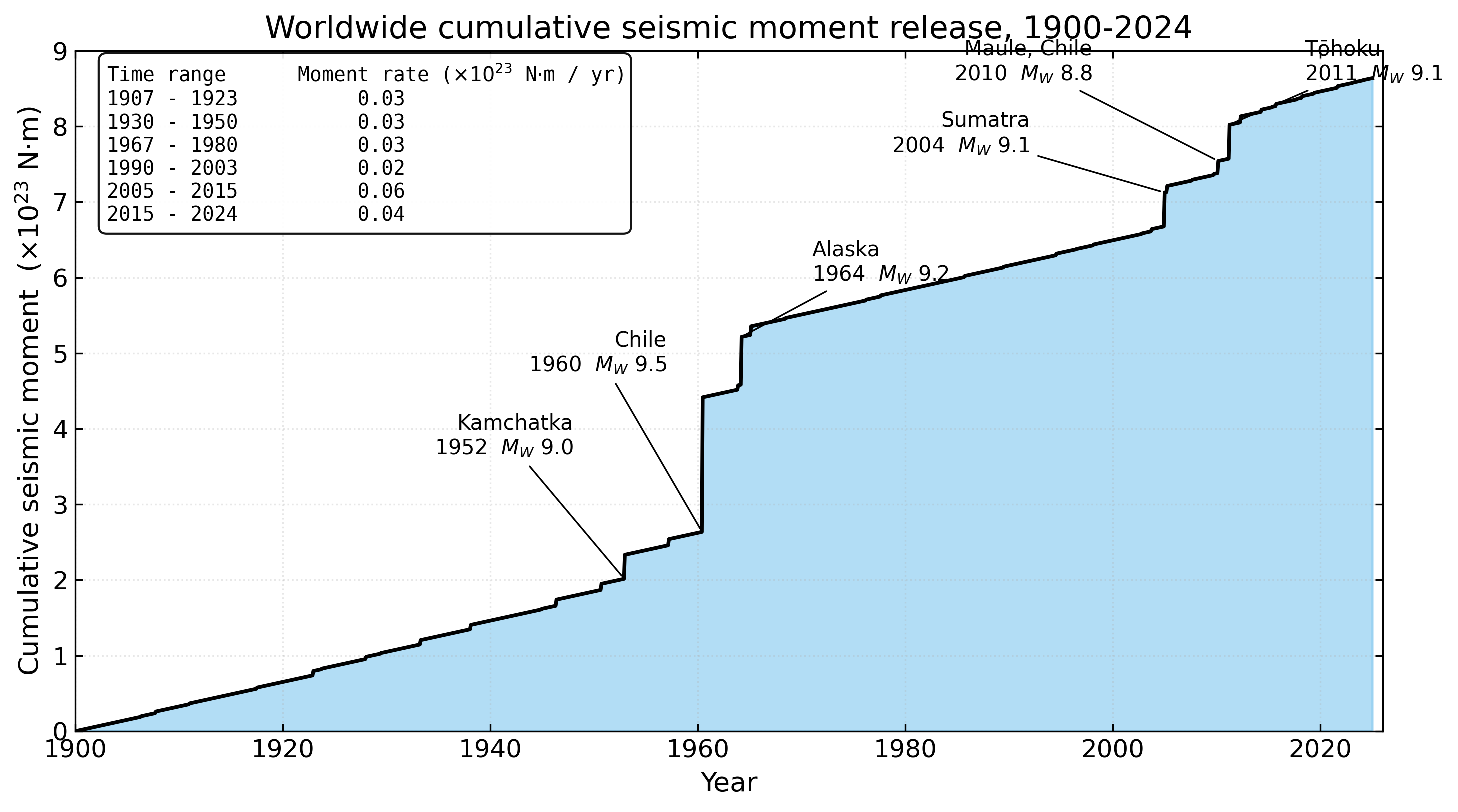
Plot of cumulative seismic moment in units of ten to the — Fig. 72 twenty-third newton-metres on the vertical axis versus year on the horizontal axis from 1900 to 2024. The curve grows roughly linearly through the early 20th century, then jumps steeply at three points: the 1952 Kamchatka M9.0 earthquake, the 1960 Chile M9.5 earthquake, and the 1964 Alaska M9.2 earthquake, the largest three jumps producing about half of the total cumulative moment. After 1964 the curve again grows roughly linearly with smaller jumps for events such as the 2004 Sumatra M9.1 and 2011 Tohoku M9.1 earthquakes, both labelled. By 2024 the cumulative moment is approximately 8 times ten to the twenty-third newton-metres. :width: 90%#

Cumulative worldwide seismic moment release since 1900. The plot makes the dominance of great earthquakes graphic: the steps at 1952 Kamchatka, 1960 Chile, 1964 Alaska, 2004 Sumatra, and 2011 Tōhoku are individual events. The decadal time-averaged moment-release rate (slope of the curve) varies by a factor of two depending on whether one of these events lies inside the averaging window. Data: USGS NEIC plus GCMT catalogues.

9. Research Horizon#

The core machinery of magnitude — equations (117), (118), (119), and (121) — is settled science. The frontier is in how these magnitudes are measured, in real time, on networks of heterogeneous instruments, and what is done with the resulting numbers operationally. The references below are deliberately drawn from the post-2020 literature so that you can see what the field is arguing about now.

Real-time moment magnitude for tsunami warning. Traditional CMT inversion takes tens of minutes after an event, by which time a tsunami may already be on its way. Goldberg et al. [2024] show that peak ground displacement (PGD) measured from real-time GNSS in the first ~30 s after origin time is a robust, non-saturating proxy for \(M_W\) that has been embedded in the USGS ShakeAlert system across the West Coast. The complementary geodetic algorithm GFAST [Pacific Northwest Seismic Network, 2024], developed at UW for PNSN, was integrated into ShakeAlert in 2024 — finally giving Cascadia a magnitude estimator that does not saturate at \(M_W\) 7.

Machine-learning detection, picking, and magnitude. Mousavi and Beroza [2022] review the rapidly expanding literature on neural-network phase pickers (PhaseNet [Zhu and Beroza, 2019], EQTransformer [Mousavi et al., 2020]) and end-to-end magnitude estimators that have lowered the magnitude of completeness in many regional catalogues by 0.5–1.0 unit, revealing the population of microseismic events that was previously below detection. The Phase Neural Operator [Sun et al., 2023] extends this to a multi- station, network-aware architecture, and the same machinery is now producing a re-trained ML catalogue for the PNSN.

ETAS and operational aftershock forecasting. The USGS Aftershock Forecast service combines a real-time fit of the Omori-law decay rate with a Gutenberg–Richter projection forward, producing a probabilistic forecast of the number of aftershocks above a given magnitude in the next day, week, and month. Recent extensions (Hardebeck et al. [2024]) use space- and time-dependent Epidemic-Type Aftershock Sequence (ETAS) triggering kernels that capture the cascade of aftershock-of-aftershock sequences that simple Omori decay misses; the same approach was used to forecast the 2023 Türkiye–Syria \(M_W\) 7.8 doublet sequence in near real time [Mai et al., 2023].

DAS, smartphone, and crowd-sourced magnitude estimation. Distributed acoustic sensing (DAS) on telecommunication fibre is now a routine seismic platform for offshore Cascadia [Wilcock et al., 2025, Zhu et al., 2023]; Yin et al. [2023] demonstrate DAS-based \(M_W\) estimation for moderate earthquakes with accuracy within 0.2 unit of the USGS catalogue. Smartphone accelerometer networks (the MyShake system [Allen et al., 2020]) now detect events with magnitudes as low as \(M_L\) 2.5 from raw phone-MEMS data and have triggered ShakeAlert-class warnings in California, Oregon, and Washington.

Beyond Earth — magnitude on Mars. The InSight lander (2018–2022) recorded the first marsquake catalogue ever assembled. Because InSight had only one station, magnitudes are reported on a Mars- specific moment-magnitude scale \(M_W^{\rm Ma}\) that uses Mars’s crustal rigidity (\(\mu \approx 25\) GPa) and a Martian distance correction [Böhm et al., 2022]. The largest event recorded, S1222a on 4 May 2022, has \(M_W^{\rm Ma} \approx 4.7\) — the largest non-impact marsquake yet observed and the first to excite detectable surface waves [Kawamura et al., 2023]. The same \(M_0 = \mu A_f \bar{s}\) relation that you applied to a Cascadia earthquake also locates Mars in the planetary seismicity hierarchy.

10. AI Literacy#

AI as a reasoning partner — checking magnitude scaling

A common point of confusion is whether “one magnitude unit means ten times bigger” or “one magnitude unit means thirty-two times bigger”. Both statements are true — but for different quantities. One magnitude unit is a factor of 10 in amplitude, a factor of \(10^{1.5} \approx 32\) in energy. Try the following with an AI assistant (Claude, ChatGPT, Gemini), and grade its answer with the rubric below.

Prompt 1 (factual). “If one earthquake has \(M_W\) 7 and another has \(M_W\) 5, by what factor is the first earthquake larger? Be specific about which physical quantity you mean.”

Prompt 2 (reasoning). “A news article states that ‘a magnitude 6 earthquake releases 10 times more energy than a magnitude 5’. Is this statement correct? If not, identify exactly what mistake the journalist made and rewrite the sentence correctly.”

Prompt 3 (calculation). “An earthquake has \(M_W\) 7.0. The fault ruptured an area of 200 km², in continental crust with rigidity 30 GPa. What is the average slip on the fault?”

Rubric. Award full credit for an answer that distinguishes amplitude, moment, and energy quantitatively (Prompt 1); identifies the factor-of-32 error and corrects “10 times more energy” to “10 times more amplitude” or “32 times more energy” (Prompt 2); and correctly derives \(\bar{s} = M_0 / (\mu A_f) \approx 1.05\) m using \(M_0 = 10^{1.5 \times 7 + 9.0} = 10^{19.5}\) N·m, \(\mu = 3 \times 10^{10}\) Pa, \(A_f = 2 \times 10^{8}\) m² (Prompt 3). Penalise any answer that reports \(\bar{s} = M_W / (\mu A_f)\) — a unit-error trap that LLMs occasionally fall into when the prompt mixes \(M_W\) and \(M_0\) vocabulary.

This activity practices LO-7 (responsible AI use) and LO-OUT-H (critique an AI explanation). The point is not that AI assistants are unreliable — they are, in fact, often correct on these problems — but that you must check the answer using the same physics you have learned, because the assistant’s confidence is uncorrelated with its accuracy on quantitative questions.

11. Concept Checks#

A regional broadband station records a peak Wood-Anderson- equivalent amplitude of 50 mm at an epicentral distance of 10 km from a Pacific Northwest earthquake. What is the local magnitude \(M_L\)? (Use the calibration: \(M_L = \log_{10} A + 3.0\) when \(A\) is in mm and \(\Delta = 100\) km, and the rule of thumb that \(-\log_{10} A_0\) at 10 km is about 1.0 unit smaller than at 100 km.)
The Tōhoku-oki 2011 earthquake had \(M_W = 9.1\). The Loma Prieta 1989 California earthquake had \(M_W = 6.9\). By what factor did Tōhoku release more seismic moment? More radiated energy?
A subduction-zone earthquake of \(M_W = 8.0\) is reported with \(M_S = 8.0\). A second event of \(M_W = 9.0\) is reported with \(M_S = 8.3\). Why is the gap between \(M_W\) and \(M_S\) much larger for the larger event?
A regional catalogue contains 1000 earthquakes per year above \(M = 3\). Assuming a Gutenberg-Richter distribution with \(b = 1\), estimate the expected number per year above \(M = 6\). How does this compare with the global rate of approximately 134 \(M \geq 6\) events per year?

12. Connections#

Backwards. This lecture builds on Lecture 14 — Earthquake Phenomena I (\(T_S - T_P\) distance, hypocentre location, focal mechanisms) and on the wave-amplitude attenuation ideas from Lectures 4–5.
Forwards. Lecture 16 — Ground Motions takes moment as the input to ground-motion prediction equations for hazard assessment, and Lecture 18 — Tsunami shows how a saturating-vs-non-saturating magnitude becomes a tsunami warning decision.
Across methods. Section 5 (forward / inverse problem) parallels Lectures 10 and 12: the long-period seismic spectrum is a forward operator for \(M_0\), and the inversion is regularised in the same sense as a tomographic inversion.
Lab. Lab 4 (in development) walks students through computing \(M_L\) from PNSN waveforms and comparing the result with the USGS catalogue \(M_W\) — the physics is what is being assessed; ObsPy takes care of waveform handling.
Discussion. Discussion 7 — Inside the Planet — uses the magnitude-depth distribution of subduction-zone seismicity to diagnose the geometry of the Wadati–Benioff zone.


Course LOs addressed	LO-1, LO-2, LO-4, LO-7
Learning outcomes practiced	LO-OUT-B (compute moment, magnitude differences, GR rates), LO-OUT-C (explain physical basis of magnitude saturation), LO-OUT-E (interpret magnitude uncertainty across scales), LO-OUT-H (critique an AI-generated explanation of magnitude vs. intensity)
Prior lecture	Lecture 14 — Earthquake Phenomena I: faults, focal mechanisms, hypocentre location
Next lecture	Lecture 16 — Ground Motions: from moment to predicted shaking and the building-code link
Lab connection	Lab 4 (in progress): students compute \(M_L\) from PNSN waveforms and compare with USGS \(M_W\)
Discussion connection	Discussion 7 — Inside the Planet (magnitude–depth distribution of subduction-zone seismicity)