Geophysics Lab 2: More Python, and Some Earthquakes

Name: Firstname Lastname

If you don’t put your name in both the spot above AND the filename, you will not receive a grade for this lab. Double-click this cell to add your name, run the cell when you’re done.

NB: In the filename, please do not put any spaces between words or wildcard characters. I access all of your submissions from my command line, and you are harshing my vibe with the spaces. Thanks!

# run this cell to import some of the packages needed to complete this lab:
import numpy as np               # more on numpy here:       https://numpy.org/doc/stable/user/absolute_beginners.html
import matplotlib.pyplot as plt  # more on matplotlib here:  https://matplotlib.org/stable/users/explain/quick_start.html

Section 1: Flex Your Python Skills

This section will focus on teaching you how to write your own script in the notebook, and further develop your skills with writing Python code. There are no problems in this section for you to solve. This section is purely to help you and act as reference.

A script or program is a series of commands executed in a row. It is much easier to write a script that can be run over and over again than to retype your code line by line. Any notebook can be treated as a script, and the cells can be run consecutively. In Python, we import specific modules that contain useful functions. This allows to not store everything in memory, but just pick and choose what we want.

Start a script in which you define a 1x10 row vector x with equally spaced values between 1 and 10.

x = np.linspace(1,10,10)
print(x)
print(x.shape)

Next, calculate the sine and cosine of vector x.

y = np.sin(x) # Remember to add comments that explain your code :)
z = np.cos(x)

Plot both functions and add a legend.

plt.figure(figsize=(10,5)) 
plt.plot(x,y, 'g-', label='sin(x)')
plt.plot(x,z, 'r-', label='cos(x)')
plt.legend()   # include the legend
plt.xlim(1,10) # limit the x axis to only the relevant area
plt.grid()     # include gridlines on the plot
plt.show();    # the ; supresses the text output about the plot from the cell. keeps your output a bit cleaner :)

Increase the smoothess of your plots by increasing the number of elements in your x vector. You can accomplish this by changing one number in your script, and then rerunning it.

x2 = np.linspace(1,10,50) # hint: the "one number" is the 50 here (the number of steps in the linspace)
y2 = np.sin(x2)
z2 = np.cos(x2)

# Let's make a quick plot to show the difference in the smoothness! 
fig, ax = plt.subplots(2,1)                                                # now we are making two images appear in one plotting output

# row 1, column 1: first plot
ax[0].plot(x, y, color='deepskyblue', label='sin(x)')                      # you can get pretty crazy with the colors!
ax[0].plot(x2, y2, color='orangered', linestyle='dotted', label='sin(x2)') # you can also dictate the line style using 'linestyle'
ax[0].set_title('Curves with Differing Smoothness')                        # title the plot
ax[0].set_ylabel('Sine of x')                                              # label the y axis for the first plot
ax[0].legend()                                                             # inlude the legend for the first plot
ax[0].grid()                                                               # gridlines for the first plot
ax[0].set_xticklabels([])                                                  # make it so we aren't labeling the x axis twice

# row 2, column 1: second plot
ax[1].plot(x, z, color='deepskyblue', label='cos(x)')                      # https://matplotlib.org/stable/gallery/color/named_colors.html
ax[1].plot(x2, z2, color='orangered', linestyle='dotted', label='cos(x2)') # ^ for the fun colors
ax[1].set_xlabel('x (radians)')                                            # label the x axis for both plots
ax[1].set_ylabel('Cosine of x')                                            # label the y axis for the second plot
ax[1].legend()                                                             # include the legend for the second plot
ax[1].grid()                                                               # gridlines for the second plot

plt.tight_layout() 
plt.show();

Section 2: Looping in Python

This section focuses on how to write an iterative method called a ‘for loop’ in Python. This section has one problem for you to solve at the end.

You can perform operations on every element of a vector or matrix at the same time, as demonstrated in Lab 1. However, sometimes you want to do something slightly different to each element, or you may just want to perform an operation multiple times. For loops enable this kind of programming. Although there are often better ways to go element-wise than a for loop, it’s still important to understand how they work and be prepared to use them. (You will end up using them. You can’t escape it. Sorry.)

Think about the command:

x1=x*4

Now, this command is absolutely how to go about multiplying every element of the vector x by the same scalar. But what if you wanted to multiply every element, going by its index? For that, we will create a for loop.

It is better practice in computing to allocate the memory the variables at the beginning of scripts. Many dynamic computing languages like Matlab, Python, Julia are flexible with on-the-fly allocations, but it slows down codes. When filling the values of the variable in a for-loop, we have to declare the variable before calling it inside the loop. Let’s get started!

Pre-allocate variables (open up some empty variables to be filled):

# remember that to fill a variable inside the loop, it has to exist before you do the loop
x  = np.arange(1,51,1)
x1 = np.zeros(50)      # this is our 'empty' variable to be filled in the loop

Now try filling in the x1 values:

# first method
print("this is the first method's output:")
for i in range(len(x)):
    x1[i] = x[i]*(i+1)       # Here we do i+1 because Python starts at 0 !!!
    print(x1[i])

print('========================~* just a little break between methods *~========================')

# second method
print("this is the second method's output:")
for i,ii in enumerate(x):    # Here 'i' is the index and 'ii' is the value of the ith index 
    x1[i] = (i+1)*ii
    print(x1[i])

In this script, the variable i is the index into the vector x. For example, when i=0, then x[i] is the first element of x (this is a Python and C++ thing, the counting starts at i=1 for Matlab and Julia).

The for loop will perform the calculation starting when i=0, then move on to i=1, etc., until it gets to the final element of the vector. In for loops, indexing is very important. Let me say that again, in case you missed it: in for loops, the indexing is VERY IMPORTANT. The command x1[i]=x[i]*4 occurs inside the for loop, and i has a different value for every pass through the loop.

Create a randomly sized matrix M with all of the elements equal to 1. Randomly determine the number of rows and columns in M using the randint() function:

# generate random integer values
from numpy.random import seed, randint # you must import these separately, from the sub-package 'np.random'

# seed random number generator
seed(1)                                # This ensures that each time you generate random numbers, you...

# ... also generate some integers
values = randint(0, 10, 20)
print(values)

# now do the matrix
seed(42)

nrows = randint(1,10,1)    # number of rows
print('number of rows:', nrows)

ncolumns = randint(1,10,1) # number of columns
print('number of columns:', ncolumns) 

This will randomly generate a number between 1 and 10 and assign them to the row and column variables.

Now, create a matrix M using the function np.ones(), with the row and column variables as inputs. The row variable should define the number of rows in M, while the column variable should define the number of columns in M.

M = np.ones([nrows[0],ncolumns[0]]) # index to take the first value, since 'nrows' and 'ncolumns' are arrays
print(M.shape)                      # prints the shape of M as (number of rows, number of columns)
print(len(M))                       # prints the 'length' of M, which is the number of rows in M

Create a set of for loops that multiplies each entry in M by the product of its row and column position. For example, the entry in the 2nd row and 3rd column should be multiplied by (2*3). Remember that Python starts indexing at 0.

# Oops! it's already done for you. Take a look:

for i in range(nrows[0]):          # outer loop
    for j in range(ncolumns[0]):   # inner loop
        M[i,j]=M[i,j]*(j+1)*(i+1)

print(M)

The above is called a ‘nested for loop’, where there is a loop inside of another loop. This means that for every single iteration of the outer loop, the inner loop must iterate until it can’t anymore, and then the action returns to the outer loop and repeats. More info here: https://pythonbasics.org/nested-loops/

Problem for Section 2

Problem 2.1: \ What is the difference between the output of the length and shape functions? Describe in words, and output the values for shape and length of M in a cell. (2 points)

Double-click this cell and replace this text with your description for Problem 2.1. Run the cell when you’re done.

# and then put your output values for the shape and length of M in the below print statements:

print("The shape of M is:", ...)   # replace the '...' with your output for the shape of M
print("The length of M is:", ...)  # replace the '...' with your output for the length of M

Section 3: Earthquake Travel Times

This section focuses on using the skills you have learned so far to calculate simple earthquake travel times. This section consists of two problems for you to solve.

You are going to practice writing a script to calculate the travel time curve of P and S waves from a shallow earthquake. Here’s some relevant information:

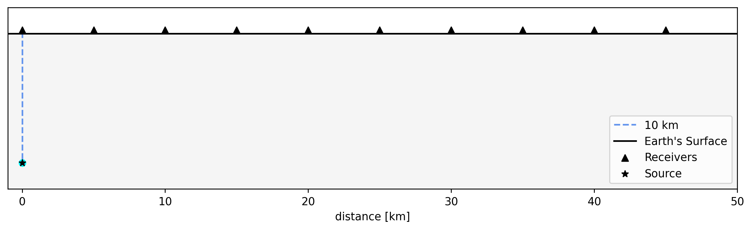
• The earthquake occurs 10 km underground, and is recorded on 10 seismometers.

• The first seismometer is directly above the earthquake.

• The second seismometer is 5 km east of the first, the third is 5 km east from the second and so on. (This setup is illustrated in the figure below.)

• The P-wave velocity for the layer is 6 km/s, and the S-wave velocity is 4 km/s.

# RUN THIS CELL and ignore the code in the cell, just look at the figure 
# I'm just making the figure for your reference

#### ignore ignore ignore ####
import numpy as np
import matplotlib.pyplot as plt

# first some vectors and values [IGNORE THESE, THEY'RE JUST FOR PLOTTING]
distance = np.linspace(-1,50,52)       # x distance, [km] 
surface  = np.zeros_like(distance)     # earth's surface
base     = -12*np.ones_like(distance)  # lower bound for the plot
receive  = np.linspace(0,45,10)        # receiver spacing
pairing  = 0.25*np.ones_like(receive)  # you need a y vector to plot the x vector
s_depth  = np.linspace(-9.7,0,10)      # source depth indicator -- IGNORE THE VALUES HERE, IT'S JUST FOR PLOTTING

# then the figure [IGNORE THIS CODE, JUST LOOK AT THE FIGURE]
plt.figure(figsize=(12,3),dpi=250)
plt.fill_between(distance, surface, base, where=surface>base, color='whitesmoke')
plt.plot(np.zeros_like(s_depth), s_depth, color='cornflowerblue',linestyle='dashed',label='10 km')
plt.plot(distance,surface,color='black',label="Earth's Surface")
plt.scatter(receive,pairing,marker='^', color='black',label='Receivers')
plt.scatter(0,-10, marker='o', color='aqua')
plt.scatter(0,-10, marker='*', color='black', label='Source')
plt.yticks([])
plt.ylim(-12,2)
plt.xlim(-1,50)
plt.legend()
plt.xlabel('distance [km]')
plt.show();

Problems for Section 3

Problem 3.1:
What is the distance between the earthquake and the third station? (You can help yourself by drawing a straight-line ray path on a paper-copy of this figure.) Solve either by hand and comment-in your work to the cell below, or use Python here in this notebook.

Define and put your answer in a float variable called solution_31. (A float is a number like 12.3 or 3.0, etc.) (3 points)

# your work (as comments) OR your code here

solution_31 = ... # replace the '...' with your answer, as a float!
solution_31

Problem 3.2:
You will now write a script to calculate and plot a travel-time curve for the seismic waves from this earthquake. Your script should do the following:

1. Define variables as follows: x is a vector containing the epicentral distance between the earthquake and each station; h is the source depth; d is a vector of source-station distances; vp and vs are the P- and S-wave speeds respectively; tp and ts for P- and S-wave travel times. Remember to comment long names for variables, and their units, into your code.

2. Calculate the travel times based on the distances and velocities.

3. Plot the travel time curves. The x axis will be the epicentral distance in km, which is defined to be the horizontal distance between the epicenter (point at surface directly above the source) and the station. The y axis will be the travel time (s) of the wave to each station. Plot both P- and S-waves on the same figure, but with different colors. Include a title and axis labels on your figure. Add a legend to the top right corner of the plot.

Comment your code. Commenting greatly helps anyone else reading your code figure out what you mean to do in each line (for instance, the person grading this…). (6 points)

# this cell is a prompt for you to solve Problem 3.2

# Type below

x  = ...       # epicentral distance vector, [units]
h  = ...
d  = ...
vp = ...
vs = ...

tp = ...
ts = ...

plt.figure(figsize = (10, 5), dpi = 100)
plt.plot(x, tp, ...)
plt.plot(x, ts, ...)
...

Section 4: Seismic Wave Ray Tracing

This section focuses on using a Python package called ‘ObsPy’ to do seismic ray tracing. This section has three problems for you to solve at the end.

P and S waves travel all over the world by traveling through the Earth. Because of changes in seismic velocity and boundaries between different layers, the ray paths can be complicated. In addition, when looking at ray paths on larger scales, we have to take into account the fact that the Earth is round(ish).

We will use Ray Tracing from the open-source software Python Obspy (for more information: https://docs.obspy.org/). Obspy provides plenty of useful built-in functions that have been validated by the community. If you need help installing ObsPy, please contact your TA.

Figure for your reference from Shearer, “Introduction to seismology” (2009), PREM velocity and density model. Additionally, you can take a look at Chapter 7, section 7.4: ‘Internal Structure of the Earth’ in your textbook (Fundamentals of Geophysics, Third Edition, by Lowrie and Fitchner), which also covers this material.

import obspy # need to import the package in order to use it

# NB: the import will not work if you don't have obspy installed. 
# !!! contact your TA if this cell returns an error !!!

First, we reproduce the results from the previous exercise

from obspy.taup import plot_travel_times

fig, ax = plt.subplots()
ax = plot_travel_times(source_depth=10, ax=ax, fig=fig, model='iasp91',
                       phase_list=['P','S'], npoints=200)

Angular distances in degrees are the angle (in degrees) from the source, to the receiver, with the point of reference located in the center of the Earth. A 90\(^\circ\) angular distance is a quarter of the Earth circumference away from the source.

You will now see the ray paths for the P, S, PKP (P wave in the outer core), and ScS (S wave reflected off the core-mantle boundary) phases as well as a travel time curve for all four phases.

from obspy.taup.tau import plot_ray_paths
from obspy.taup import TauPyModel


model   = TauPyModel(model='iasp91')
fig, ax = plt.subplots(subplot_kw=dict(polar=True))       # this declares the figure variables
fig.set_size_inches(18,10)                                # this sets the size of the figure
ax = plot_ray_paths(source_depth=100, ax=ax, fig=fig, phase_list=['P','S', 'PKP','ScS'], 
                    npoints=25,show=False,legend=True)    # this is a built-in function to plot the rays
ax.set_title('Ray tracing in a spherical Earth')          # this will add a title

# the below lines will add text on the plot
ax.text(0, 0, 'Solid\ninner\ncore',
        horizontalalignment='center', verticalalignment='center',
        bbox=dict(facecolor='white', edgecolor='none', alpha=0.7))
ocr = (model.model.radius_of_planet -
       (model.model.s_mod.v_mod.iocb_depth +
        model.model.s_mod.v_mod.cmb_depth) / 2)
ax.text(np.deg2rad(180), ocr, 'Fluid outer core',
        horizontalalignment='center',
        bbox=dict(facecolor='white', edgecolor='none', alpha=0.7))
mr = model.model.radius_of_planet - model.model.s_mod.v_mod.cmb_depth / 2
ax.text(np.deg2rad(180), mr, 'Solid mantle',
        horizontalalignment='center',
        bbox=dict(facecolor='white', edgecolor='none', alpha=0.7))
plt.show();

Problems for Section 4

Problem 4.1:
Why aren’t there any S waves in the outer core? (2 points)

Double-click this cell and replace this text with your answer to Problem 4.1. Run the cell when you’re done

Problem 4.2:
Notice that within the mantle (the first thick layer), the ray paths of both the P and S waves are curved. What causes this curvature? Think about what happens to the seismic velocity with increasing depth and the cause of this phenomenon. Remember seismic velocity depends on more than just density. (3 points)

Double-click this cell and replace this text with your answer to Problem 4.2. Run the cell when you’re done

Problem 4.3:
What direction do the P-waves bend as they enter the outer core? What does this say about the P-wave velocity in the outer core vs. the mantle? (2 points)

Double-click this cell and replace this text with your answer to Problem 4.3. Run the cell when you’re done

Section 5: Challenge Section! Triplications in the Crust

This section expands on the content in Section 4. There is one problem in this section for you to solve, but it is extra credit.

Below we will see why once we can detect several P waves. We calculate the ray paths and travel time at really short distances, for an earthquake a source depth of 5km and a distance of about 111 km (1\(^\circ\) of angular distances).

# this cell might take a second to run

model = TauPyModel(model='prem')

# plot the travel-time curves
fig,ax  = plt.subplots()
fig.set_size_inches(10,6)
ax = plot_travel_times(source_depth=5, ax=ax, fig=fig, model='prem',
                       phase_list=['P'], npoints=200, max_degrees=1.5, min_degrees=0)
ax.grid(True)
ax.set_title('Travel-time curves')
print('')


# plot the ray paths in cartesian coordinates.
arrivals = model.get_ray_paths(5, 1, phase_list=['P'])
arrivals.plot_rays(plot_type='cartesian', phase_list=['P'],
                   plot_all=False, legend=True)
plt.show();

Extra Credit Challenge Problem for Section 5

Problem 5.1:
What are the 3 different P wave phases that cause the triplication?

You don’t need to know the specific notation (e.g. PKP), but you should be able to explain what they are, based on what you have been learning in class and the material they are traveling through. Look at the depth of the plot, and be specific. (2 points)

Double-click this text and replace it with your answer to Problem 5.1. Run the cell when you’re done.

Due on Wednesday, April 15 at 5:00 pm

Submission instructions:
Make sure you have run all cells in your notebook, in order, before saving and submitting, so that all images/graphs appear in the output in your submission. Save the final version of this notebook with your name in the filename and at the beginning (where there is a spot for it). Upload a copy of your notebook to Canvas by Wednesday, April 15 at 5:00 pm.

This concludes Lab 2.

Congrats, you made it!